Foreword

The present notes are the lecture notes for the course of Algebraic Geometry in Bristol the second teaching block in 2023/2024. We mainly follow the book of Karen Smith et al. “An Invitation to Algebraic Geometry ((Smith et al. 2000))” but also add other examples, exercises, and topics from other sources. We have several copies of this book in the Maths library in Queens Building. Our other references are

• Joe Harris, Algebraic Geometry, A First Course, (Harris 1995)

• Atiyah and Macdonald, Introduction to commutative algebra, (Atiyah and Macdonald 1969)

• Miles Reid, Undergraduate algebraic geometry, (Reid 1988)

• Robin Hartshorne, Algebraic geometry, (Hartshorne 1977)

• Shafarevich, Basic Algebraic Geometry, (Shafarevich 1974)

1 Closed Affine Algebraic Varieties

1.1 Definition and Examples

Algebraic geometry is the area of mathematics where the relation between algebraic objects, mostly an ideal of polynomials of several variables over a field, and the corresponding geometric object, the zero loci of the polynomials is investigated. These geometric objects are called algebraic varieties. One goal is to be able to read off the geometric properties of a given algebraic variety from the algebraic data on its ideal. For instance, this course will show how irreducibility, dimension, and singularities can be defined purely algebraically.

In recent years, interest in computational aspects of algebraic geometry has grown, and also we have seen many applications of algebraic geometry in all the other areas of mathematics, such as combinatorics. This has led to the subject of combinatorial algebraic geometry which includes toric and tropical geometry. Time permitting, we discuss the basics of these theories and make an effort to describe many algebro-geometric properties of some algebraic varieties from the combinatorial data.

1.2 Closed Affine Algebraic Varieties in \(\mathbb{C}^n\)

We first define the basic notion of closed affine algebraic varieties. For our course, we mainly consider the field of complex numbers as our ground field and look at the common zero loci of \(n\)-variable polynomials in \(\mathbb{C}^n,\) but from time to time we mention whether the theorems hold in other fields or not.

1.3 The Zariski Topology on \(\mathbb{C}^n\)

We intend to define a topology on \(\mathbb{C}^n\) where the closed sets are the (closed affine) algebraic varieties. We verify immediately after stating the definition that these closed sets do indeed give rise to a topology.

2 Algebraic Foundations

2.1 A bit of Algebra

We recall some basic definitions from Ring Theory and Commutative Algebra. We trust that the reader knows the definition of rings, fields, modules, and vector spaces on their own. Gladly, all the rings in this course are commutative and contain multiplicative identity element \(1.\) Let \(R\) be a ring, recall that a nonempty subset \(I\subseteq R\) is called an ideal, if for all \(a, b \in I\) and \(r \in R,\) we have \[a+b \in I,~ ra \in I.\] For any subset \(J \subseteq R,\) the ideal generated by \(J\) is given by \[(J) =\bigcap \big\{\text{all ideals in $R$ containing $J$} \big\},\] Note that \((J)\) is an ideal; the intersection of any collection of ideals is still an ideal. The reader can verify that \((J)\) is all the linear combinations of elements of \(J\) with coefficients in \(R,\) i.e., \[(J) = \big\{r_1 j_1 + \dots + r_k j_k : \text{for any positive integer } k,\, j_i \in J,\, r_i \in R \big\}.\] An ideal \(I\) is finitely generated, if there are finitely many elements \(f_1, \dots, f_k \in I\) such that \[(f_1,\dots, f_k ) = (\{f_1,\dots, f_k \}) = I.\]

Given an ideal \(I\subseteq R\), we can define the quotient ring \(R/ I.\) The elements of \(R/ I\) are the cosets of \(I.\) The map \(\pi: R \longrightarrow R / I,\) \(r \longmapsto r+ I,\) is a surjective ring homomorphism. Note under the map \(\pi,\) an ideal \(K\subseteq R\), which contains \(I\) is mapped to an ideal of \(R/ I.\) Conversely, if \(J \subseteq R/ I\), is an ideal, then the preimage \(\pi^{-1}(J)\) is an ideal in \(R\) containing \(I.\) As a result:

Recall also that:

Assume that \(\alpha: Q \longrightarrow R,\) is a ring homomorphism, that is, it preserves sums, products, and maps any multiplicative or additive identity element in \(Q\) to a multiplicative or additive identity element in \(R\), respectively. If \(\mathfrak{p}\subseteq R\) is prime, then \(\alpha^{-1}(\mathfrak{p})\subseteq Q\) is also prime. To see this, note that \[\bar{\alpha}: Q \longrightarrow R/ \mathfrak{p},\] is a ring homomorphism, and we have \[\ker{\bar{\alpha}} =\alpha^{-1}(\mathfrak{p})\] and \(Q/ \ker{\bar{\alpha}}\) is isomorphic to a subring of \(R/ \mathfrak{p}\). As a result, \(Q / \ker{\bar{\alpha}}\) is an integral domain, and \(\alpha^{-1}(\mathfrak{p})\) is also prime. When \(\mathfrak{m}\subseteq R\) is maximal, \(\alpha^{-1}(\mathfrak{m})\) is certainly prime, however, not necessarily maximal. (Example: \(Q:= \mathbb{Z}, R:= \mathbb{Q}, \mathfrak{m}= (0).\)) Let \((R, + , .)\) be a ring and \(\mathbb{K}\) be a field. If \((R, + )\) is also a \(\mathbb{K}\)-vector space, then \(R\) is called a \(\mathbb{K}\)-algebra.

Analogously to the case of rings and ideals, one defines:

2.2 Hilbert’s Basis Theorem

In this section, we show that every algebraic variety can be described as the zero loci of finitely many polynomials.

We leave it to the reader to verify that the above two definitions of Noetherian property are equivalent. Note that every field is Noetherian since it has only the ideals \((0)\) and \((1).\) Therefore, the following theorem immediately implies that \[\mathbb{C}[x_1, \dots , x_{n-1} , x_n] = (\mathbb{C}[x_1, \dots , x_{n-1} ])[x_n]\] is a Noetherian ring.

2.3 The Ideal of a Variety and Nullstellensatz

For a subset \(A \subseteq \mathbb{A}^n,\) we define the ideal corresponding to \(A\), denoted by \(\mathbb{I}(A)\), as the set \[\mathbb{I}(A) := \{f \in \mathbb{C}[x_1, \dots, x_n] : f(x) = 0 \text{ for all } x\in A\}.\] That is, the set of all the polynomial functions vanishing on \(A.\) It is clear that \(\mathbb{I}(A)\) is an ideal in \(\mathbb{C}[x_1, \dots , x_n].\) For every \(A\), \(\mathbb{I}(A)\) is, in fact, radical: If \(f^n(x)=0\) for some integer \(n>0\) and all \(x \in A,\) then \(f(x)=0\) for all \(x\in A.\)

By Hilbert’s Basis Theorem 2.9, \[I = \mathbb{I}(A)= (f_1, \dots , f_k),\] for some positive integer \(k,\) and \(f_i\in \mathbb{C}[x_1, \dots , x_n].\) Now, if we moreover assume that \(V\) is a closed affine algebraic variety, then \[\mathbb{V}(\mathbb{I}(V)) = V.\] To see this,

• If \(x\in V,\) then \(f(x) =0\) for all \(f\in \mathbb{I}(V)\) and \(x \in \mathbb{V}(\mathbb{I}(V)).\)

• If \(x\in \mathbb{V}(\mathbb{I}(V)),\) then \(f(x)=0\) for all \(f\in \mathbb{I}(V).\) But \(V\) is an algebraic variety and is given by \(V = \mathbb{V}(\{g_i\}_{i\in A})\) for some \(g_i \in \mathbb{C}[x_1, \dots ,x_n]\). Thus, \(g_i\in \mathbb{I}(V),\) and \(\mathbb{V}(\mathbb{I}(V))\subseteq \mathbb{V}(\{g_i\}_{i\in A}).\)

Now we can use Hilbert’s Basis Theorem 2.9 to show that

“Any closed affine algebraic variety is an intersection of finitely many closed affine algebraic hypersurfaces.”

Now a natural question arises: Do we also have the equality \(\mathbb{I}(\mathbb{V}(I)) = I \,?\) To experiment, let us take \(V = \{1 \}\subseteq \mathbb{C}= \mathbb{A}^1.\) On the one hand, for the ideal \(I:= (x-1)^2,\) we have \(\mathbb{V}(I)= \{1 \}.\) On the other hand, \(f(x)=x-1 \in \mathbb{I}(V),\) but \(f\notin I.\) The following theorem answers our question:

In German Nullstellen = zero set + Satz = theorem. Miles Reid in (Reid 1988) recommends that one should stick to the German word if they don’t want to be considered an “ignorant peasant”.

Note that \(V \subseteq W \subseteq \mathbb{A}^n,\) if and only if, \(\mathbb{I}(W) \subseteq \mathbb{I}(V).\) Thus, Hilbert’s correspondence between ideals and varieties is inclusion-reversing.

Now observe that, on the one hand, the smallest, with respect to inclusion, closed affine algebraic varieties are single points. Therefore, the correspondence implies that the points correspond to the maximal ideals in \(\mathbb{C}[x_1, \dots, x_n]\). On the other hand, the ideals of the form \(\mathfrak{m}_{a}= (x_1 - a_1,\dots , x_n -a_n)\) are maximal: define the surjective ring homomorphism \(\delta_a: \mathbb{C}[x_1, \dots, x_n] \longrightarrow\mathbb{C},\) \(\delta_a(f) := f(a).\) Then \(\mathfrak{m}_a = \ker(\delta_a)\). As \(\mathbb{C}\) is a field, \(\mathfrak{m}_a\) has to be maximal. By definition, \(\mathfrak{m}_a \subseteq \mathbb{I}(\{a\}),\) \(\mathbb{I}(\{a\}) \neq \mathbb{C}[x_1, \dots, x_n]\), therefore, \(\mathfrak{m}_{a} = \mathbb{I}\{a\}.\) As a result, \[a= (a_1,\dots , a_n)\in \mathbb{A}^n \longleftrightarrow \mathfrak{m}_{a} = (x_1 - a_1,\dots , x_n -a_n).\]

2.4 Irreducibility and Dimension

We now notice that the ‘indecomposibility’ of prime ideals has a geometric meaning.

In summary, for \(A:= \mathbb{C}[x_1,\dots,x_n]\)

Now we state the following decomposition theorem.

The above properties allow for defining the dimension of closed affine algebraic varieties:

We accept the following theorems:

2.4.1 An application: Cayley–Hamilton Theorem

As an application, we can prove the Cayley–Hamilton Theorem, borrowed from the beautiful notes of Edixhoven and Taelman (Edixhoven and Taelman 2009), which I have uploaded on Blackboard.

2.5 Morphisms of Closed Affine Algebraic Varieties

A polynomial map \[\begin{align*} \varphi: \mathbb{A}^n &\longrightarrow\mathbb{A}^m, \\ a & \longmapsto\varphi(a) = (\varphi_1(a), \dots, \varphi_m(a)), \end{align*}\] where all \(\varphi_i\)’s are polynomials in \(n\) variables. More generally, we have the notion of a morphism of algebraic varieties.

2.6 The Coordinate Ring

We have that

“\(\mathbb{C}[V]\) is a \(\mathbb{C}\)-algebra and can be viewed as the set of all the polynomial functions in \(\mathbb{C}[x_1, \dots, x_n]\) restricted to \(V.\)”

To see the above statement, note that \(\mathbb{C}[V]\) is a \(\mathbb{C}\)-algebra and that the restriction \[\begin{align*} \mathbb{C}[x_1, \dots, x_n] &\longrightarrow\mathbb{C}[x_1, \dots, x_n]_{|_{V}}, \\ f & \longmapsto f_{|_V}. \end{align*}\] is a surjective \(\mathbb{C}\)-algebra homomorphism with kernel \(\mathbb{I}(V).\)

Recall that a ring is called reduced if it has no non-zero nilpotent elements.

2.7 Affine Schemes

In this section, we explain the correspondence \(\mathbb{C}[V] \leftrightarrow V\) and will try to understand the idea behind the notion of the affine schemes. For a ring \(R\), let us define the maximal spectrum of \(R\) by \[\textrm{maxSpec}(R) = \{\mathfrak{m}\subseteq R : \text{$\mathfrak{m}$ is a maximal ideal} \}.\] In the following paragraphs, we discuss that for any closed affine algebraic variety \(V \subseteq \mathbb{A}^n,\) \(\textrm{maxSpec}(\mathbb{C}[V])\) can be endowed with the Zariski topology, and can be identified with \(V.\) To warm up, note that all the maximal ideals of \(A:= \mathbb{C}[x_1, \dots, x_n]\) are of the form \(\mathfrak{m}_a = (x_1-a_1, \dots, x_n - a_n),\) where \(a= (a_1, \dots, a_n)\) is a point in \(\mathbb{A}^n.\) As any subset of \(\mathbb{A}^n\) is the union of its points, combined with Nullstellensatz, and Exercise 2.14⁴, we obtain: \[\mathbb{V}(I) = \bigcup_{a\in \mathbb{V}(I)} \{a\} \quad \longleftrightarrow \quad \mathbb{I}(\mathbb{V}(I)) = \sqrt{I}= \bigcap_{\mathfrak{m}_a \supseteq I} \mathfrak{m}_a.\] Moreover, for an ideal \(I\subseteq A,\) let \(V= \mathbb{V}(I):\) \[\text{maxSpec}(\mathbb{C}[V]) \quad \longleftrightarrow \quad \{ \mathfrak{m}\in \textrm{maxSpec}(A): \mathfrak{m}\supseteq \mathbb{I}(V)\} \quad \longleftrightarrow \quad \{\text{points in $\mathbb{V}(I)$}\}.\] Analogously,

• We can now define the Zariski closed sets of \(\textrm{maxSpec}(A)\). Recall that the Zariski closed sets in \(\mathbb{A}^n\) are \[\begin{multline*} \mathbb{V}(I) = \{a \in \mathbb{A}^n: f(a)=0, \text{$f\in I$}\} \\ = \{a \in \mathbb{A}^n: f\in \mathfrak{m}_a, \text{$f\in I$}\} \\ = \{a \in \mathbb{A}^n: \mathfrak{m}_a \supseteq I\}, \end{multline*}\] for \(I \subseteq A\) an ideal. Similarly define the Zariski topology on \(\textrm{maxSpec}(A)\) by declaring the closed sets to be \[\mathbb{V}(I) = \{\mathfrak{m}\in \textrm{maxSpec}(A): \mathfrak{m}\supseteq I \},\] for any ideal \(I\subseteq A.\) Similarly, we can define the Zariski topology on \(\textrm{maxSpec}\big(\mathbb{C}[V] \big)\) by declaring the closed sets to be \[\textcolor{blue}{\mathbb{V}(J) = \{\mathfrak{m}\in \textrm{maxSpec}\big(\mathbb{C}[V] \big): \mathfrak{m}\supseteq J \}},\] for ideals \(J \subseteq \mathbb{C}[V].\)

• For a morphism of algebraic varieties \(\varphi: V \longrightarrow W,\) we can consider the pullback \(\varphi^*: \mathbb{C}[W] \longrightarrow\mathbb{C}[V].\) If \(a\in V \longmapsto\varphi(a) \in W,\) and \(a\) and \(\varphi(a)\) correspond to the maximal ideals \(\mathfrak{m}_a \subseteq \mathbb{C}[V]\) and \(\mathfrak{n}_{\varphi(a)} \subseteq \mathbb{C}[W],\) respectively. We have \[(\varphi^*)^{-1}(\mathfrak{m}_{a})= \mathfrak{n}_{\varphi(a)}.\] To see this, note that \[\begin{multline*} f \in \mathfrak{n}_{\varphi(a)} \iff f(\varphi(a)) = 0 \iff \varphi^*(f) (a) =0\\ \iff \varphi^*(f) \in \mathfrak{m}_{a} \iff f\in (\varphi^*)^{-1}(\mathfrak{m}_{a}). \end{multline*}\] That is, the inverse image of the maximal ideals in this case is maximal. To summarise into a diagram:

  

  As a result, any homomorphism \(\Phi:R \longrightarrow S\) of finitely generated reduced \(\mathbb{C}\)-algebras induces a continuous map of associated maximal spectra \[\Phi^{-1}: \textrm{maxSpec}(S) \longrightarrow\textrm{maxSpec}(R).\]

In summary, the Nullstellensatz for \(\mathbb{C}[x_1,\dots , x_n]\) and Theorem 2.39, the above Properties (a),(b) allow for turning \(\textrm{maxSpec}(R)\) to a nice topological space when \(R\) is finitely generated reduced \(\mathbb{C}\)-algebra. However, it is impossible to replace \(\mathbb{C}[V]\) in the above definition by any commutative ring, since in general the inverse image of a maximal ideal is not necessarily maximal. The profound idea in Scheme Theory is that changing the concentration from the maximal ideals to the prime ideals⁵ makes this generalisation possible:

The spectrum of the ring seems like a natural generalisation of \(\textrm{maxSpec}\), but since our points are the prime ideals now, peculiar situations appear as we show in the examples below. Note that maximal ideals still correspond to points, but these points are closed since the smallest closed set containing \(\mathfrak{m},\) the closure of \(\mathfrak{m}\) equals \(\mathbb{V}(\mathfrak{m})=\{\mathfrak{m}\}.\)

Example 2.48. Compared to \(\textrm{maxSpec}(\mathbb{C}[x])\), the spectrum \(\mathrm{Spec}(\mathbb{C}[x])\) has a spooky new guest \((0)\). The closed points correspond to the maximal ideals which are of the form \((x-a)\), \(a\in \mathbb{C}.\) Therefore, the closed points do correspond to a specific point \(a\in \mathbb{C},\) but \((0)\) cannot be placed anywhere, and at the same time “near” to every other point. See Figure 1.1.

2.8 The Equivalence of Algebra and Geometry

In the language of the categories, the results in Section 2.6 can be rephrased as the equivalence of the following two categories:

• \(\textsf{Var}:=\) the category of (closed affine) algebraic varieties;

• \(\textsf{Alg}_{\mathbb{C}}:=\) the category of finitely generated, reduced \(\mathbb{C}\)-algebras.

Roughly speaking, a category has objects and morphisms between any pairs of objects. Morphisms are also called maps or simply arrows. For \(\textsf{Var}\) the objects are the varieties, and the morphisms are the morphisms of algebraic varieties. For \(\textsf{Alg}_{\mathbb{C}}\) the objects are the reduced, finitely generated \(\mathbb{C}\)-algebras, and the morphisms are \(\mathbb{C}\)-algebra homomorphisms. Every object \(A\) in a category \(\textsf{C}\), is associated with an identity morphism \(\text{id}_A\). In each category, there is a natural composition of morphisms that is associative. A functor is a map between two categories. More precisely, A covariant functor \(\mathscr{F}\) from a category \(\textsf{C} = (\textrm{Obj}(\textsf{C}), \textrm{Mor}(\textsf{C}))\) to the category \(\textsf{D} = (\textrm{Obj}(\textsf{D}), \textrm{Mor}(\textsf{D}))\), denoted by \(\mathscr{F}: \textsf{C} \longrightarrow\textsf{D},\) consists of the information

• A map of objects \(\textrm{Obj}(\textsf{C}) \longrightarrow\textrm{Obj}(\textsf{D});\)

• A map of morphisms \(\textrm{Mor}(\textsf{C}) \longrightarrow\textrm{Mor}(\textsf{D}),\)

satisfying

• For every object \(A \in \textsf{C},\) \(\mathscr{F}(\text{id}_A) = \text{id}_{\mathscr{F}(A)};\)

• If

  

  then

  

  is also commutative.

A contravariant functor reverses the arrows. For any category \(\textsf{C}\) we can naturally define the identity functor \(\mathrm{id}_{\textsf{C}},\) which allows us to define the important notion of the equivalence of categories. We say that the two categories \(\textsf{C}\) and \(\textsf{D}\) are equivalent if there are functors \(\mathscr{F}: \textsf{C} \longrightarrow\textsf{D},\) and \(\mathscr{G}: \textsf{D} \longrightarrow\textsf{C},\) such that \[\mathscr{G}\circ \mathscr{F} \simeq \text{id}_{\textsf{C}}\, , \quad \mathscr{F}\circ \mathscr{G} \simeq \text{id}_{\textsf{D}}.\] That is, for any \(A\in \textrm{Obj}(\textsf{C}),\) the object \(\mathscr{G} \circ \mathscr{F}(A)\in \textrm{Obj}(\textsf{C})\) is an object isomorphic to \(A\) (and not necessarily equal). This holds true similarly for \(\mathscr{F}\circ \mathscr{G}.\) Now let us define the functor \[\begin{align*} \mathscr{F}: \textsf{Var} &\longrightarrow\textsf{Alg}_{\mathbb{C}}, \\ \textrm{Obj}(\textsf{Var}) \ni V &\longmapsto\mathscr{F}(V):= \mathbb{C}[V] \in \textcolor{blue}{\textrm{Obj}(\textsf{Alg}_{\mathbb{C}})} , \\ \textrm{Mor}(\textsf{Var}) \ni \varphi &\longmapsto\mathscr{F}(\varphi):= \varphi^* \in \textrm{Mor}(\textsf{Alg}_{\mathbb{C}}). \end{align*}\] Also, \[\begin{align*} \mathscr{G}: \textsf{Alg}_{\mathbb{C}} &\longrightarrow\textsf{Var}, \\ \textrm{Obj}(\textsf{Alg}_{\mathbb{C}}) \ni \mathbb{C}[V] &\longmapsto\mathscr{G}(V):= \textrm{maxSpec}(\mathbb{C}[V]), \\ \textrm{Mor}(\textsf{Alg}_{\mathbb{C}}) \ni \Phi &\longmapsto\mathscr{G}(\Phi)=\varphi, \end{align*}\] where \(\varphi\) is defined in Theorem 2.39(b). The results in Section 2.6 verify that

• \(\mathscr{F}\) is a functor;

• \(\mathscr{G}\) is a functor;

• \(\mathscr{G}\circ \mathscr{F} \simeq \text{id}_{\textsf{Alg}_{\mathbb{C}}},\) and \(\mathscr{F}\circ \mathscr{G} \simeq \text{id}_{\textsf{Var}}.\)

In summary, we have the equivalence between \(\textsf{Var}\) and \(\textsf{Alg}_{\mathbb{C}}.\) This equivalence also highlights a very modern view in mathematics: often, to study sets, we study the functions on them. In our case,

“Studying polynomial functions on algebraic varieties provides enough information to understand algebraic varieties up to isomorphism.”

The reader interested in learning more on Category Theory may consult nice and gentle notes of Tom Leinster (Leinster 2014) which are available at https://arxiv.org/pdf/1612.09375.pdf, or very solid notes of Pierre Schapira (Schapira 2023).

3 Projective Varieties

3.1 Projective Space

In this section, we define the projective spaces. A projective space of dimension \(n\) contains a copy of \(\mathbb{A}^n,\) and it turns out to be a compact set in the Euclidean topology. Let us set \(\mathbb{C}^* = \mathbb{C}\setminus \{0\}.\)

Let us note the following.

• The equivalence relation means \(\mathbb P^n\) corresponds to the set of all lines in \(\mathbb{C}^{n+1},\) passing through the origin. Therefore, any element or point in \(\mathbb P^n\) corresponds to such a line.

• A point \(a\in \mathbb P^n\) is a class of points in \(\mathbb{C}^{n+1}\setminus \{0\}\) under the equivalence relation. In coordinates, such a point is denoted by \(a=[x_0: \dots : x_n],\) which are called the homogeneous coordinates of \(a\).

• The equivalence relation \(\sim\) can be understood by the orbits of the action of \(\mathbb{C}^*\) on \(\mathbb{C}^{n+1}\setminus \{ 0\}\) by \((\lambda , a)\longmapsto\lambda \cdot a.\) That is, \(a\sim b\) if and only if \(a\) and \(b\) lie on the same orbit under the action of \(\mathbb{C}^*.\)

• The above projective space can be defined over any field \(k.\) Moreover, when \(k= \mathbb{R},\) then \[\mathbb{R}\mathbb P^n = (\mathbb{S}^n)/ \sim,\] where \(\mathbb{S}^n = \{x\in \mathbb{R}^{n+1}: \lVert x \rVert =1 \}\) is the \(n\)-dimensional sphere, and \(a\sim b\) if and only if \(a = \pm b.\) Note that \[\mathbb{S}^n = (\mathbb{R}^{n+1}\setminus \{0\}) / \sim_1\] where \(\sim_1\) is the equivalence relation that \(a \sim_1 b\) if and only if \(a = \lambda \, b\) for \(\lambda >0.\)

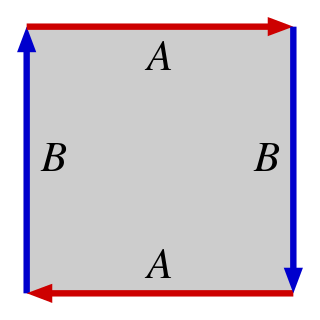
Exercise 3.3. Convince yourself that the real projective plane \(\mathbb{R}\mathbb P^2\) is a disc with the sides identified as in Figure 1.3.

For completeness let us recall the definition of an analytic manifold; see (Voisin 2002).

3.1.1 A Quick Review: Complex Analysis in One Variable

A function \(f: U \longrightarrow\mathbb{C}\), where \(U \subseteq \mathbb{C}\) is an open set, is said to be differentiable at a point \(z_0 \in U\) if the limit \[f'(z_0) = \lim_{z \to z_0} \frac{f(z) - f(z_0)}{z - z_0}\] exists.

The first big surprise of the theory of complex functions, which has no direct analogue for real functions \(g: \mathbb{R}^2 \to \mathbb{R}^2\), is the following:

Exercise 3.12.

• Derive the Cauchy–Riemann equations from the picture below and Theorem 3.10.

• Write \(\frac{\partial f}{\partial x} = \frac{\partial u}{\partial x} + i \frac{\partial v}{\partial x}\) and \(\frac{\partial f}{\partial y} = \frac{\partial u}{\partial y} + i \frac{\partial v}{\partial y}\) \[\frac{\partial f}{\partial \bar{z}} = \frac{1}{2} \left( \frac{\partial f}{\partial x} + i \frac{\partial f}{\partial y} \right) =0.\] Thus \(\frac{\partial f}{\partial \bar{z}}\) measures how far \(f\) is from being analytic.

The following implies that by having the values of holomorphic \(f\) around the point \(z_0\), you can determine \(f(z_0).\)

3.2 Projective Varieties

Let \(f(x_0,x_1) = x_0 +x_1 -1.\) First observe that the variety \(\mathbb{V}(f)\) defines a line in \(\mathbb{C}^2.\) However, in \(\mathbb P^1\) such a zero set is not well-defined, since \([x_0, x_1]\in \mathbb P^1\) has to be exactly the same point as \([\lambda x_0, \lambda x_1]\) for any \(\lambda \in \mathbb{C}^*.\) But \(x_0 + x_1 =1\) does not imply that \(\lambda x_0 + \lambda x_1 = 1\) for all \(\lambda \in \mathbb{C}^*.\) On the other hand, observe that \(\mathbb{V}(x_0^3 + x_0 x_1^2 + x_1^3)\) is, in fact, well-defined in \(\mathbb P^1.\) These observations prompt us to concentrate on the polynomials whose zero sets are invariant under the \(\mathbb{C}^*\)-action, and as we will see in Proposition 3.19, are exactly the homogeneous polynomials, i.e., a polynomial that all of its monomial summands have the same degree. Now it is easy to see that if \(h\in \mathbb{C}[x_0, \dots , x_n],\) is a homogeneous polynomial of degree \(d\), then \[h(\lambda x_0, \dots , \lambda x_n) = \lambda^d h(x_0, \dots , x_n),\] has a well-defined zero locus on the projective space.

Now we have two ways to understand any projective variety using the affine varieties:

• By using the affine charts. For instance, we have \(\mathbb P^n = \bigcup_{i=0}^{n} U_i,\) where \(U_i\) were defined in Theorem 3.6. Therefore, \[V =\bigcup_{i=0}^{n} ( V \cap U_i) \subseteq \mathbb P^n.\] Note that \(U_i\)’s are only one choice of affine charts for \(\mathbb P^n.\)

• By the affine cone over the variety. The affine cone is obtained by looking at the zero set of the homogenous polynomial equations defining \(V= \mathbb{V}(\{f_i \}_{i\in I})\) in \(\mathbb{C}^{n+1}.\) Intuitively, we can consider \(\mathbb P^n \subseteq \mathbb{A}^{n+1},\) (as a subset and not an algebraic subvariety), and for every point in \(V\subseteq \mathbb P^n,\) assign the line from the origin passing through that point.

3.3 The Homogeneous Nullstellensatz

We intend to use the quotient map \(q:\mathbb{A}^{n+1} \setminus \{0\} \longrightarrow\mathbb P^n\), to define a topology on \(\mathbb P^n.\) That is easy: the Zariski topology on \(\mathbb{A}^{n+1}\) induces a topology on \(\mathbb{A}^{n+1}\setminus \{0\},\) which in turn, induces a quotient topology on \(\mathbb P^n,\) i.e., the unique topology on \(\mathbb P^n\) that makes \(q\) a continuous map. In other words, \[\begin{multline*} Y \subseteq \mathbb P^n \text{ is closed } \iff q^{-1}(Y ) \subseteq \mathbb{A}^{n+1} \setminus \{0\} \text{ is closed } \\ \iff \exists \, Z \subseteq \mathbb{A}^{n+1} \text{ closed, such that } q^{-1}(Y ) = Z \cap (\mathbb{A}^{n+1} \setminus \{0\}). \end{multline*}\] Therefore, we have the bijection \[\begin{align*} \label{eq:bij-torus-inv} \big\{\text{closed subsets of $\mathbb P^n$ }\big\} &\xrightarrow{\simeq} \big\{ \text{closed $\mathbb{C}^*$-invariant subsets of $\mathbb{A}^{n+1}$ containing $0$} \big\}, \\ Y &\mapsto q^{-1}(Y) \cup \{0\}. \end{align*}\] By Nullstellensatz, the closed subsets of \(\mathbb{A}^{n+1}\) correspond to the radical ideals in \(\mathbb{C}[x_0, \dots, x_n].\) So we ask ourselves, what are the ideals that correspond to the \(\mathbb{C}^*\)-invariant subsets? Let us discuss the situation with an illuminating example.

Motivated by the above example, we define the following.

Let \(\mathfrak{m}_0 = (x_0 -0 , \dots , x_n - 0)\) denote the maximal ideal corresponding to \(0 = (0,\dots , 0) \in \mathbb{A}^{n+1},\) which does not belong to \(\mathbb P^{n}.\)

The preceding proposition justifies the following definition, and proves that it coincides with the quotient topology from \(\mathbb{A}^{n+1}.\)

We have also the following correspondence:

More precisely,

3.4 The Projective Closure of an Affine Variety

Recall from Example 3.2, that we viewed \(\mathbb P^1\) as \(\mathbb{C}\cup \{\infty\}.\) We have \[\mathbb P^1 = \begin{cases} U_0:= \{ [1: x_1 /x_0] \} = \{[1: a]: a\in \mathbb{C}\} & \text{if $x_0\neq 0$}; \\ \{ [0: x_1]: x_1 \neq 0 \}= \{ [0: 1]\} & \text{if $x_0= 0$}. \end{cases}\] Obviously, \(x_0\) is a homogeneous polynomial and \(\mathbb{V}(x_0)\) is closed in \(\mathbb P^1.\) Therefore, its complement \(U_0\) is open in \(\mathbb P^1.\) We can now ask what is the closure of \(U_0\) in \(\mathbb P^1?\) The answer is \(\mathbb P^1,\) since the smallest closed set in \(\mathbb P^1\) containing \(U_0\) is \(\mathbb{V}(0).\) To see this, assume that \(\mathbb{V}(I)\subseteq \mathbb P^1\) is the closure of \(U_0,\) then if \(g(x_0,x_1) \in I,\) then \(g_{|_{U_0}}\) is a polynomial in \(\mathbb{C}[a]\) vanishing on \(U_0 \simeq \mathbb{A}^1.\) Therefore, it has to be zero! Now we can ask a more general question. Assume \(V \subset \mathbb{A}^n,\) and we have identified \(\mathbb{A}^n\) as above with \(U_0\). What is the closure of \(V\subseteq U_0\) in \(\mathbb P^n?\) This set is called the projective closure of \(V\). Before stating the main theorem, let us go through another example: let \(\ell := \{(a,b): a+b+1 =0 \}\subseteq \mathbb{A}^2.\) To find the closure \(\overline{\ell}\subseteq\mathbb P^2,\) note that if \(\overline{\ell}= \mathbb{V}(g),\) for \(g\in \mathbb{C}[x,y,z],\) then \(g\) must be a homogeneous polynomial such that \(g_{|_{U_0}}\) vanishes on \(\ell.\) So a good candidate for \(g\) is \(x+y+z,\) because on \(U_z,\) \(z\neq 0\) and \([x:y:z] = [x/z: y/z :1].\) By replacing \(a = x/z\) and \(b = y/z,\) we must have \(a+b+1 =0\) on \(\ell.\) Note that \((x+y+z) (x)\) or \((x+y+z)^2\) also vanish on \(\ell\) when we restrict them to \(U_z\) but they are not ‘minimal’. We can alternatively identify \(U_z = \{z\ne 0 \}\) with the points where \(z=1,\) by choosing one representative of \(U_z\) and think that \[x+y+z_{|_{U_z}}= x+y+1.\] Note also that \(x+y+z\) even though it has a well-defined zero set in \(\mathbb P^2,\) it is not a function \(\mathbb P^2 \longrightarrow\mathbb{C},\) but when we fix a representative on \(U_z,\) then it becomes an honest function! We now need a general procedure to go from \(x+y+1\) to \(x+y+z.\) This process is called homogenisation, and it is very simple:

For instance, homogenising \(x + y + z^3 + 4xy\) gives \(x u^2 + y u^2 + z^3 + 4xyu\), which is obtained by compensating for the lower-degree terms with powers of a new variable.

Note that if a variety \(V = \mathbb{V}(I) \subseteq \mathbb{A}^n\) is defined by an ideal \(I \subseteq \mathbb{C}[x_1, \dots, x_n]\), then by Hilbert’s Basis Theorem, there exist finitely many generators \(I = (g_1, \dots, g_k)\), and we have \(V = \mathbb{V}(g_1, \dots, g_k)\). However, in general, as Example 3.35 below shows, we do not necessarily have \[\overline{V} = \mathbb{V}(\tilde{g_1}, \dots, \tilde{g_k}).\] Thus, while \(\mathbb{I}(\overline{V}) \subseteq \mathbb{C}[x_0, \dots, x_n]\) is finitely generated, the polynomials \(\tilde{g_1}, \dots, \tilde{g_k}\) may not form a generating set. The following theorem, however, shows that one way to find the closure is to homogenise all the elements of the ideal \(I\) and consider their common zero set.

3.5 Morphisms of Projective Varieties

In Section 1.4 we explain how to define a good notion of “coordinate rings" for projective varieties by glueing ‘local’ ones.

3.6 Why do we care about the Projective Varieties?

It is easy to see that projective spaces are compact with respect to the induced Euclidean topology from \(\mathbb{A}^{n+1}.\) Therefore, their Zariski closed subsets, the projective varieties, are also compact with respect to the Euclidean topology. Compactness properties simplify many theorems. For instance, two distinct lines in \(\mathbb P^2\) always meet at exactly one point, which is not true in the affine case. There are also many topological properties of projective varieties, which are not true in the affine case. Several important conjectures, such as Grothendieck Standard Conjectures and The celebrated Hodge Conjecture are proposed in the projective case. Let us mention the following two important theorems that only hold in the projective setting.

Chow’s Lemma certainly does not hold in the affine case. For instance, \(\mathbb{V}(y -e^x)\) is an affine analytic variety, and it cannot be described as a zero set of any polynomial equation. Chow Lemma has been generalised enormously by Jean-Pierre Serre in a famous article known as GAGA.

Before ending this chapter, let us define the notion of dimension and degree for projective varieties.

4 Quasi-Affine and Quasi-Projective Varieties

In other words, a quasi affine (respectively quasi-projective) variety is a locally closed subset of \(\mathbb{A}^n\) (respectively \(\mathbb P^n\)). Recall that in a topological space \(X\), a set \(V\) is called locally closed, if there exists an open subset \(U \subseteq X\) and a closed subset \(Z\subseteq X,\) such that \(V = U \cap Z.\) From now on, the word variety means any affine, quasi-affine, projective, or quasi-projective variety.

4.1 Regular Functions

For a few sections, we mainly follow (Hartshorne 1977)*Section I.3.

4.1.1 Regular Functions on Quasi-Affine Algebraic Varieties

Now, if you have taken the course of Algebraic Geometry to only care about polynomial functions, you might not be happy to see the regular functions. However,

• The local nature of regular functions is essential in algebraic geometry for glueing the pieces of affine algebraic varieties;

• (Global) regular functions on affine algebraic varieties (and not only proper open subsets) and projective algebraic varieties, do behave like polynomial functions as we will see in Theorems 4.7, 4.14.

4.1.2 A Basis for Zariski Topology of Affine Varieties

Recall that a basis for a topology is a collection \(\mathcal{B}\) of open subsets of a topological space \(X\) such that every open set \(U\) in \(X\) can be written as a union of a collection of elements in \(\mathcal{B}\). Note that for any polynomial \(f\in \mathbb{C}[x_1,\dots , x_n],\) the set \[D(f) := \mathbb{A}^n \setminus \mathbb{V}(f),\] is an open subset in \(\mathbb{A}^n.\) Note that \(D(f_1) \cup D(f_2) = \big( \mathbb{A}^n \setminus \mathbb{V}(f_1) \big) \cup \big( \mathbb{A}^n \setminus \mathbb{V}(f_2) \big) = \mathbb{A}^n \setminus (\mathbb{V}(f_1) \cap \mathbb{V}(f_2)).\) As a result, if \(I = (f_1, \dots , f_k) \subseteq \mathbb{C}[x_1, \dots , x_n]\) is an ideal, then \[\mathbb{A}^n \setminus \mathbb{V}(I) = \bigcup_{i=1}^{k} D(f_i).\] In consequence, the sets of the form \(D(f)\) form a basis for the Zariski topology of \(\mathbb{A}^n.\) Replacing \(A^n\) with \(V= \mathbb{V}(g_1, \dots , g_{\ell})\subseteq \mathbb{A}^n\), we can simply check that the sets of the form \(V\cap D(f) = V \setminus \mathbb{V}(f)\) for \(f\in \mathbb{C}[x_1, \dots ,x_n]\) or equivalently \(D(g)\) for \(g \in \mathbb{C}[V],\)⁹ also form a basis for any closed affine algebraic variety \(V.\)

4.1.3 Regular Functions on Quasi-Projective Algebraic Varieties

The following definition is, in fact, equivalent to Definition 3.37, for projective varieties.

We state the following theorem without proof, which implies that regular functions on projective spaces are very restricted.

We leave the proof of the following theorem as an exercise.

We can easily generalise the preceding example to show that:

“Any open subset \(D(f)\subseteq \mathbb{A}^n\) is isomorphic to a closed subset of \(\mathbb{A}^{n+1}.\)”

Namely, \[\begin{align*} \varphi: D(f)= \mathbb{A}^n \setminus \mathbb{V}(f) &\longrightarrow\mathbb{A}^{n+1} \\ (x_1, \dots , x_n) &\longmapsto\Big(x_1, \dots , x_n , \frac{1}{f(x_1, \dots , x_n)}\Big), \end{align*}\]

• \(\varphi(D(f))\) is closed in \(\mathbb{A}^{n+1};\)

• \(\varphi: D(f) \longrightarrow\varphi(D(f))\) is a morphism.

To see these, assume that \(\mathbb{A}^{n+1}\) has the coordinates \((x_1, \dots , x_n, z).\) We have

• \(\varphi(D(f)) = \mathbb{V}(z f -1);\)

• Since \(x_1,\dots, x_n, f(x_1, \dots , x_n)\) are all regular functions on \(D(f),\) \(\varphi\) is a morphism by Theorem 4.15.

It is also easy to check that \[\begin{align*} \psi: \mathbb{V}(zf -1 ) &\longrightarrow D(f) \\ (x_1,\dots, x_n,z) &\longmapsto(x_1, \dots , x_n) \end{align*}\] is a morphism and the inverse to \(\varphi.\) More generally, similar to above, we can show that if \(V= \mathbb{V}(g_1, \dots , g_{\ell}),\) the open subset \[D(f)\cap V = \mathbb{V}(g_1, \dots , g_{\ell})\setminus \mathbb{V}(f),\] is isomorphic to \(W:= \mathbb{V}(g_1, \dots , g_\ell , zf -1).\) By Theorem 4.7, \(\mathcal{O}_V(V) = \mathbb{C}[V] = \frac{\mathbb{C}[x_1, \dots , x_n]} {\mathbb{I}(V)}= \frac{\mathbb{C}[x_1, \dots , x_n]} {(g_1, \dots , g_{\ell})},\) and we can understand the coordinate ring \[\begin{multline*} \mathbb{C}[D(f)\cap V] := \mathbb{C}[V]_{f} := \frac{\mathbb{C}[x_1, \dots , x_n, 1/f]}{(g_1, \dots , g_\ell)} = \varphi^*(\mathbb{C}[W])\\ \simeq \mathbb{C}[W] = \frac{\mathbb{C}[x_1, \dots , x_n, z]} {(g_1, \dots , g_{\ell}, zf-1 )}. \end{multline*}\] Note that by the above isomorphism, we have \[\mathcal{O}_V[D(f) \cap V] = \varphi^* (\mathcal{O}_W(W)) = \varphi^* (\mathbb{C}[W]) \simeq \mathbb{C}[V]_{f}.\]

Summary of this section

• We defined quasi affine/projective varieties: open subsets.

• Found a basis for Zariski topology on c.a.a.v \(V\subseteq \mathbb{A}^n\): open subsets of the form \(D(f):= V \setminus \mathbb{V}(f),\) for \(f\in \mathbb{C}[V].\)

• Defined regular functions: roughly, \(f(x)/g(x)\) on open subsets, where \(g\) doesn’t vanish. We needed \(f,g\) to be of the same degree in the projective case.

• Defined isomorphism in general: continuous maps and pulling back regular to regular.

• Found the regular functions on closed affine algebraic varieties and their open basis: \[\mathcal{O}_V(V)= \mathbb{C}[V], \quad \mathcal{O}_V(D(f))= \mathbb{C}[V]_{f}= \mathbb{C}[V, 1/f] = \frac{\mathbb{C}[x_1, \dots, x_n, z]}{(\mathbb{I}(V), zf-1)}.\]

4.2 Two Examples of Glueing

4.2.1 Obtaining \(\mathbb P^1\)

We have seen in Example 3.2.(e) that we can construct \(\mathbb P^1\) by glueing two copies of \(\mathbb{A}^1\) along \(\mathbb{A}^1 \setminus \{0\},\) by the map \(x\longmapsto x^{-1}.\) Let us write this more formally. We have,

• \(\xi_0: U_0 \longrightarrow X_0 := \xi_0(U_0),\) \(\xi_1: U_1 \longrightarrow X_1:= \xi_1(U_1),\) are isomorphisms.

• \(X_{01}:= \xi_0(U_0 \cap U_1) \subset X_0.\)

• \(X_{10}:= \xi_1(U_1 \cap U_0) \subset X_1.\)

• \(g_{01}:= \xi_1 \circ \xi_0^{-1}: X_{01} \longrightarrow X_{10}, \quad x \longmapsto y= x^{-1}.\)

Note that all these sets are open subsets of \(\mathbb P^1\) and isomorphic to affine algebraic varieties. We have

• \(\mathbb{C}[X_0]= \mathcal{O}_{X_0}(X_0) = \mathbb{C}[x]\), \(\mathbb{C}[X_1]= \mathcal{O}_{X_1}(X_1) = \mathbb{C}[y].\)

• \(\mathbb{C}[X_{01}]= \mathcal{O}_{X_0}(X_{01}) =\frac{\mathbb{C}[x, x']}{(xx'-1)} \simeq \mathbb{C}[x, x^{-1}]\supseteq \mathbb{C}[x].\)

• \(\mathbb{C}[X_{10}]= \mathcal{O}_{X_1}(X_{10}) = \frac{\mathbb{C}[y, y']}{(yy'-1)} \simeq \mathbb{C}[y, y^{-1}]\supseteq \mathbb{C}[y].\)

We have now the isomorphism of \(\mathbb{C}\)-algebras induced by \(\varphi:\) \[\begin{align*} g_{01}^*: \mathbb{C}[X_{10}] &\longrightarrow\mathbb{C}[X_{01}] \\ f & \longmapsto f\circ g_{01}=f(y^{-1}) \\ y & \longmapsto x= y^{-1}. \end{align*}\] Therefore, we can also think of \(\mathbb P^1\) as \(X_0\simeq \mathbb{A}^1\) and \(X_1\simeq \mathbb{A}^1,\) where \(X_{01}\) and \(X_{10}\) are glued by the isomorphism \(g_{01}.\)

4.2.2 Obtaining \(\mathbb P^2\)

Let \([x_0:x_1:x_2]\) denote the homogeneous coordinates of the space \(\mathbb{P}^2\). It is covered by three coordinate charts:

• \(U_0\) corresponding to \(x_0 \neq 0\), with affine coordinates \((\frac{x_1}{x_0}, \frac{x_2}{x_0}) = (a_1, a_2).\)

• \(U_1\) corresponding to \(x_1 \neq 0\), with affine coordinates \((\frac{x_0}{x_1}, \frac{x_2}{x_1}) = (a_1^{-1}, a_1^{-1}a_2).\)

• \(U_2\) corresponding to \(x_2 \neq 0\), with affine coordinates \((\frac{x_0}{x_2}, \frac{x_1}{x_2}) = (a_2^{-1}, a_1 a_2^{-1}).\)

As before, let \(X_i = \xi_i (U_i),\) and \(X_{ij}= \xi_{i}(U_i \cap U_j).\) We have \(\mathbb{C}[X_0]= \mathcal{O}_{X_0}(X_0) = \mathbb{C}[a_1, a_2],\) and \(\mathbb{C}[X_{01}]= \mathcal{O}_{X_0}(X_{01}) = \mathbb{C}[a_1^{-1},a_1, a_2].\) Since on \(X_1,\) \(a_1\neq 0,\) we can write \[\mathbb{C}[X_1]= \mathcal{O}_{X_1}(X_1) = \mathbb{C}[a_1^{-1}, a_1^{-1} a_2].\] As a result, \[\mathbb{C}[X_{10}]= \mathcal{O}_{X_{10}}(X_{10}) = \mathbb{C}[a_1, a_1^{-1}, a_1^{-1} a_2].\] The isomorphism

provides the information for glueing of \(X_{01}\simeq \mathbb{C}^* \times \mathbb{C}\) and \(X_{10}\simeq X_{01}\simeq \mathbb{C}^* \times \mathbb{C}\) and their corresponding coordinate rings. We can similarly understand the isomorphisms between other charts. Torus Actions¹⁰:

• On \(U_0 \ni a= (a_1, a_2)\) the action of \(t= (t_1, t_2) \in (\mathbb{C}^*)^2\) is obtained by \(t\cdot a = (t_1 a_1, t_2 a_2).\)

• On \(U_1 \ni b= (b_1, b_2)\) the action of \(t= (t_1, t_2) \in (\mathbb{C}^*)^2\) is obtained by \(t\cdot b = (t_1^{-1} b_1, t_1^{-1} t_2 b_2).\)

• On \(U_2 \ni c= (c_1, c_2)\) the action of \(t= (t_1, t_2) \in (\mathbb{C}^*)^2\) is obtained by \(t\cdot c = (t_2^{-1} c_1, t_1 t_2^{-1} c_2).\)

This is compatible with the glueing.

4.2.3 Abstract Varieties: Two Perspectives

General abstract varieties can be defined in two ways.

• Defining the abstract varieties similar to manifolds: an abstract variety has a set of functions that behave like regular functions, and each point has an open neighbourhood that is isomorphic to an affine algebraic variety. I’d like to compare this to how a structural engineer analyses a building structure.

• Defining the abstract varieties with glueing data: an abstract variety is given as \[X:= \bigsqcup X_{i}/\sim,\] where \(X_i\)’s are affine algebraic varieties, such that in their intersections we have compatible glueing data and isomorphisms between \(X_i \cap X_j \subseteq X_i\) and \(X_j \cap X_i \subseteq X_j,\) to define the equivalence or glueing. For instance, in the example of \(\mathbb P^2\) above, if the sets \(X_i\)’s and \(g_{ij}\)’s were given as the initial data, we could glue them to construct \(\mathbb P^2.\) I’d like to call this an architect point of view.

We discuss the second point of view in more detail in the chapter on Toric Varieties. These two points of view are, in fact, equivalent. See for instance https://stacks.math.columbia.edu/tag/00AK, and the details of these two constructions in the lecture notes of Edixhoven and Taelman (Edixhoven and Taelman 2009) on Blackboard.

5 Smoothness and Tangent Spaces

Consider the analytic curve \(\mathbb{V}(y-\sin(x)) \subseteq \mathbb{A}^2.\) The Taylor expansion around \(x_0=0,\) is given by \[\sin(x) = x - \frac{x^3}{3!} + \frac{x^5}{5!}- \dots.\] Therefore, the first-order approximation of \(\sin(x)\) is \(x\) and the third-order approximation is \(x - (x^3)/6,\) which are shown in the figures below.

The first-order approximation by an affine linear space, having the same dimension as our variety or manifold, defines what is known as the tangent space. Consider, for example, an affine algebraic variety \(V = \mathbb{V}(f) \subseteq \mathbb{A}^n\). Intuitively, the tangent space to \(V\) at a point \(p \in V\) is the affine linear subspace that best approximates \(V\) at \(p\).

Formally, a vector \(v \in T_p V\) if and only if the point \(a + \lambda v\) closely approximates a point in \(V\). In other words, as we slightly move along \(v\), the value \(f(a+\lambda v)\) stays near zero. Hence, we have: \[v\in T_a V \iff (Df(a)) v = \langle \nabla f(a), v \rangle = \left.\frac{d}{d\lambda}\right|_{\lambda=0} f(a+\lambda v) = 0.\]

The gradient \[\nabla f(a) = \left(\frac{\partial f}{\partial x_1}(a), \dots, \frac{\partial f}{\partial x_n}(a)\right)\] is perpendicular to the tangent space. If \(V = \mathbb{V}(f_1,\dots,f_k)\subseteq \mathbb{A}^n\), then the tangent space at \(a\) is the intersection: \[T_a V = \bigcap_{i=1}^{k} \ker(\nabla f_i(a)).\]

Formally, we state:

5.1 Smoothness

We state the following without proof:

5.2 Tangent Spaces: Algebraic Definition

(Until Chapter 6) We intend to state an intrinsic and an algebraic definition of the tangent spaces in terms of ideals. To start, as usual, we first define this concept for (closed) affine algebraic varieties. Let \(A:= \mathbb{C}[x_1, \dots , x_n],\) \(I = \mathbb{I}(V) \subseteq A,\) a radical ideal, and for a point \(a= (a_1, \dots , a_n) \in V \subseteq \mathbb{A}^n,\) denote by \(\mathfrak{m}:= \mathfrak{m}_a \subseteq A,\) the ideal corresponding to \(a \in \mathbb{A}^n,\) and \(\bar{\mathfrak{m}}:= \bar{\mathfrak{m}}_a \subseteq \mathbb{C}[V] = \frac{A}{\mathbb{I}(V)}\simeq \mathcal{O}_V(V),\) the ideal corresponding to \(a \in V.\) For any \(\mathbb{C}\)-vector space \(S,\) we denote its linear dual by \[V^* = \mathrm{Hom}(S, \mathbb{C}) = \{\text{linear functions from $S$ to $\mathbb{C}$}\}.\]

We now want to show that the tangent space can be understood completely in the algebraic setting:

• \(\mathfrak{m}_a / \mathfrak{m}_a^2\) as a \(\mathbb{C}\)-vector space, can be identified with \((T_a \mathbb{A}^n)^{*}\simeq \mathbb{A}^n;\)

• \(\bar{\mathfrak{m}}_a / \bar{\mathfrak{m}}_a^2\) as a \(\mathbb{C}\)-vector space, can be identified with \((T_a V)^{*}.\)

In order to show these claims we consider the following binary operation or pairing, \[\begin{align*} \langle \cdot , \cdot \rangle : \mathfrak{m}\,\times\,T_a\mathbb{A}^n &\longrightarrow\mathbb{C}\, , \\ (f, v ) & \longmapsto\frac{\partial f}{\partial v}(a). \end{align*}\]

6 Desingularisation and Blowing up

(This chapter) In the field of Algebraic Geometry, two varieties are considered to be birationally equivalent if they are isomorphic except for a “small set" of points. Heisuke Hironaka in 1964 proved that any quasi-projective variety over \(\mathbb{C}\) can be transformed into a smooth quasi-projective variety through a process called the blowing-up (i.e. zooming in), in other words, any quasi-projective variety can be desingularised. We discuss the blowing up process in the following paragraphs. A video lecture on this topic is available at https://youtu.be/Gkkh_nl7ETw.

6.1 Blowing up of \(\mathbb{A}^n\) at a Point

6.1.1 Blowing up \(\mathbb{A}^2\) at a Point: Intuition

We intend to discuss the following without proof:

Let us explain the idea behind the blowing up method by considering \(C:= \mathbb{V}(y^2 -x^2(x+1))\subseteq \mathbb{A}^2.\) Here is what we can do to blow up \(C:\)

• Note that the tangent space is not well-defined at the origin, but it is well-defined when we approach the origin. So we remove the origin.

• Lift any point \((a,b) \in C\setminus \{(0, 0)\}\) to the height equal to the slope of the line passing through \((a,b)\) and the origin, i.e., \((a,b) \longmapsto(a,b, \frac{b}{a}) \in (C\setminus \{(0,0)\} ) \times \mathbb{C}.\)

• Take the closure of the curve we obtained in \(\mathbb{A}^3.\)

If you’d like to look at the blowup curve from different angles, here is the Maple code.

intersectplot(u^2 = x + 1, y = x*u, x = -2 .. 2, y = -2 .. 2,
u = -2 .. 2, shading = "z", thickness = 7, 
labelfont = ["TimesNewRoman", 40]);

Now let us apply the same procedure as above to the disc.

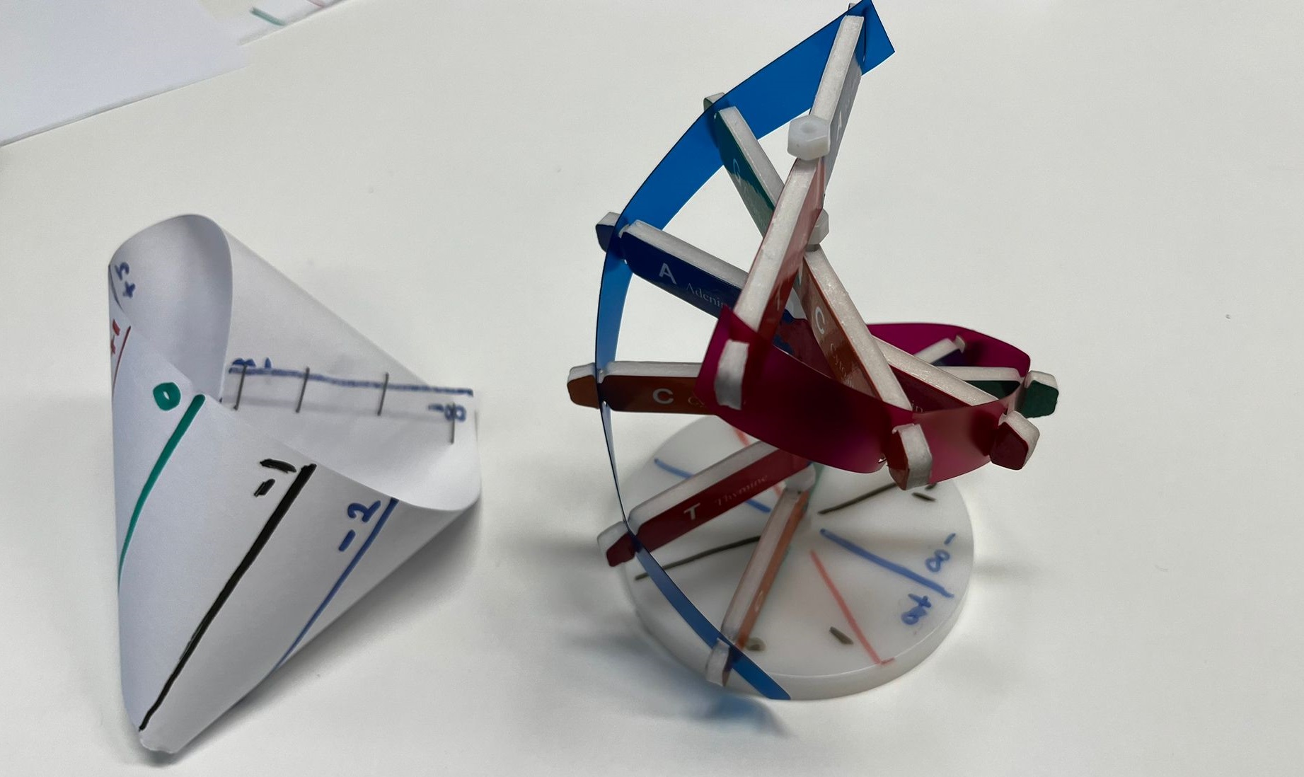
6.1.2 The Algebraic Definition

The idea for blowing up is to think that the objects we obtained above in \(\mathbb{A}^2 \times \mathbb{A}^1\) as an open chart of \(\mathbb{A}^2 \times \mathbb P^1.\) For instance consider the points \[\big((a,b); [1: \frac{b}{a}] \big)\in \mathbb{A}^2 \times \mathbb P^1,\] and extend the definition to the other chart with the usual identification \([a/b:1] = [a:b] =[1:b/a],\) when \(a\neq 0, b\neq 0.\) However, this is still not defined at \((a,b) = (0,0).\) The idea is to install an entire copy of \(\mathbb P^1\) at \((0,0).\) Another way to formulate this blowup is to think that \(\mathbb P^1\) is the set of equivalence classes of lines passing through the origin and that the point \([1: b/a]\) can be understood as the equivalence class of the line which contains the point \((a,b) \in \mathbb{A}^2.\) This leads us to define the blowup of \(\mathbb{A}^2\) at \((0,0)\) by: \[\big\{(p, [\ell]): p\in \ell \text{ for all points } p\in \mathbb{A}^2, \text{ and lines } \ell \text{ passing through $(0,0)$} \big\},\] where \([\ell] \in \mathbb P^1\) denotes the equivalence class of \(\ell.\) Note that above \((0,0)\) we get a representative of all the lines passing through the origin: \(\mathbb P^1.\) This contains the \(u\) -axis or the “slope axis" as an open affine chart, and it is called the exceptional divisor.

Now we can easily generalise this idea to any dimensions: if \(p=( x_1, x_2, \dots , x_n)\in \mathbb{A}^n\) and \(\ell = [y_1: y_2 : \dots : y_n]\in \mathbb P^{n-1},\) we have that \((x_1, x_2, \dots, x_n) \in \ell\) if and only if the vectors \((x_1, x_2, \dots, x_n),\) \((y_1, y_2, \dots , y_n) \in \mathbb{A}^n\) are along the same line or linearly dependent. In other words, \[\begin{align*} & \text{rank} \begin{pmatrix} x_1& x_2 &\cdots& x_n \\ y_1& y_2 &\cdots & y_n \end{pmatrix} \leq 1 \\ &\iff \text{determinant of all $2\times 2$-matrices vanish} \\ & \iff \{x_iy_j - y_ix_j=0: 1 \leq i, j \leq n \}. \end{align*}\] We now arrive at the following natural equivalent definitions.

h_1 := intersectplot(u^2 - x = 0, y = x*u, x = -2 .. 2, 
y = -2 .. 2, u = -2 .. 2, shading = "z", 
thickness = 7, labelfont = ["TimesNewRoman", 40]);
h_2 := intersectplot(x = 0, y = 0, x = -2 .. 2,
y = -2 .. 2, u = -2 .. 2, color = "red");
display(h_1, h_2);

6.2 Blowing up of \(\mathbb{A}^n\) along a variety

Let us briefly mention the definition of blowup of \(\mathbb{A}^n\) along an affine subvariety. Compare to Exercise 6.7. We encourage the readers to go through beautifully written Chapter 7 of (Smith et al. 2000).

7 Toric Geometry

Toric geometry is a subfield of algebraic geometry, where we can construct algebraic varieties from combinatorial and discrete data. The goal is to be able to read algebro-geometric properties of these varieties from the combinatorial data. Miles Reid in 1983, writes “This construction has been of considerable use within algebraic geometry in the last 10 years...and has also been amazingly successful as a tool of algebro-geometric imperialism, infiltrating areas of combinatorics." Fulton writes “toric varieties have provided a remarkably fertile testing ground for general theories."

7.1 Cones and their dual

Let \(N\) be a group isomorphic to \(\mathbb{Z}^n,\) i.e., a finitely generated free abelian group of rank \(n.\)

• \(N \simeq \mathbb{Z}^n\) as groups.

• The dual lattice \(M:= \mathrm{Hom}_{\mathbb{Z}}(N, \mathbb{Z}),\) i.e., all the group homomorphisms \(f:N \longrightarrow\mathbb{Z}.\)

• \(N_{\mathbb{R}}:= \mathbb{R}\otimes_{\mathbb{Z}} N.\)

• \(M_{\mathbb{R}}:= \mathbb{R}\otimes_{\mathbb{Z}} M.\)

• We have \(M \simeq \mathbb{Z}^n\) as groups, \(N_{\mathbb{R}} \simeq M_R \simeq \mathbb{R}^n\) as vector spaces. We have the natural inclusion \(M \subseteq M_{\mathbb{R}}.\)

If we identify \(N_{\mathbb{R}}= \mathbb{R}^n,\) then \(M_\mathbb{R}\) would be identified with the dual of \(\mathbb{R}^n\), denoted by \((\mathbb{R}^n)^*.\) We can denote by \(\langle \cdot , \cdot \rangle\) the pairing of \((\mathbb{R}^n)^*\) and \(\mathbb{R}^n\). This pairing is simply the dot product on \(\mathbb{R}^n,\) if we identify \((\mathbb{R}^n)^*\) and \(\mathbb{R}^n.\)

Recall that a convex cone or simply a cone \(\sigma \subseteq \mathbb{R}^n\) satisfies,

• \(v\in \sigma,\) \(\lambda \in \mathbb{R}_{\geq 0} \implies \lambda \, v \in \sigma;\)

• \(v,v' \in \sigma\) \(\implies\) \(v+v' \in \sigma.\)

In these notes, all cones are assumed to be convex.

It is easy to see the following:

Note that any cone can be understood as the intersection of half-spaces containing it. This helps us identify the dual cones easily: For \(v \in \mathbb{R}^n\) let us define \[H_v^+ = \textrm{cone}(\{v\})^{\vee} := \{u\in (\mathbb{R}^n)^*: \langle u , v \rangle \geq 0 \}.\] Now, by definition, \[\sigma^{\vee} = \bigcap_{v \in \sigma} H_v^+,\] and since \(\sigma^{\vee}\) is also convex, if \(\sigma = \textrm{cone}\{v_1, \dots , v_k\},\) \[\sigma^{\vee} = \bigcap_{i=1}^{k} H_{v_i}^+.\]

We leave the proof as an exercise.

7.2 Monoids

We are interested in additive properties of \(\sigma \cap \mathbb{Z}^n,\) where \(\sigma\) is a cone, which make it a monoid.

Note that for a monoid we only have the notion of the addition of its elements, which gives rise to the following notion.

7.3 Affine Toric Varieties

In this section, we describe how to every rational cone \(\sigma \subseteq \mathbb{R}^n,\) we can assign an affine variety \(X_{\sigma} \subseteq \mathbb{A}^N\) which is unique up to isomorphism (usually \(n \neq N\)).

We can now easily verify that for \(m_1, m_2 \in \mathbb{Z}^n,\) \[\begin{align*} m_1 & \longmapsto z^{m_1} \\ m_2 & \longmapsto z^{m_2} \\ m_1 + m_2 & \longmapsto z^{m_1 + m_2} = z^{m_1} z^{m_2}. \end{align*}\] This implies that if we have finitely many \(\{m_1 , \dots , m_k\}\) generating a monoid \(S_{\sigma},\) i.e., with different combinations of their sums, then \(z^{m_1}, z^{m_2}, \dots , z^{m_n}\) generate \(\mathbb{C}[S_{\sigma}]\) as a \(\mathbb{C}\)-algebra. Let us clarify this with some examples.

In view of the Equivalence of Algebra and Geometry in Section 2.8, the following lemma is crucial.

The preceding lemma allows for the following definition.

Let us make the following important remark.

7.3.1 Cartesian Product of Affine Algebraic Varieties

Let \(I = (f_1, \dots , f_k) \subseteq \mathbb{C}[z_1, \dots , z_n]\) and \(J = (g_1, \dots , g_{\ell}) \subseteq \mathbb{C}[t_1, \dots , t_m],\) be two radical ideals. Then, \[\mathbb{V}(I) \times \mathbb{V}(J) = \mathbb{V}(f_1, \dots , f_k , g_1, \dots , g_{\ell}) \subseteq \mathbb{A}^n \times \mathbb{A}^m\] With the coordinate ring given by \(\frac{\mathbb{C}[z_1, \dots , z_n, t_1, \dots , t_m]}{(f_1, \dots , f_k , g_1, \dots , g_{\ell}) } = \mathbb{C}[V] \otimes_\mathbb{C}\mathbb{C}[W],\) with the induced Zariski topology on \[\text{maxSpec}( \mathbb{C}[V] \otimes_\mathbb{C}\mathbb{C}[W]).\]

7.3.2 More Examples

The preceding example leads to the following question: Question. Given \(m_1=(a,b), m_2= (c,d) \in \mathbb{Z}^2,\) how can we make sure that they generate \(\textrm{cone}(\{m_1, m_2\})\) as a monoid? Answer. Check whether or not \[\det \begin{pmatrix} a& b \\ c & d \end{pmatrix} = \pm 1.\] See Exercise 7.31.

Here is a nice exercise to know when you have a set of generators and in fact works for any dimension.

Exercise 7.32. In Figure 1.9, find a set of generators for \(\textrm{cone}( \{-e_2, 3e_1+2e_2\})\cap \mathbb{Z}^2\) and the relations between these generators.

7.4 Abstract Varieties and Glueing Data

We now intend to create new varieties using existing ones. This process resembles the glueing in topology. To achieve this, we require some data for the glueing process, which includes:

1. A set \(I\);

2. For each \(i \in I\), an affine algebraic variety \(X_i\);

3. For each pair \(i, j \in I\), an open subvariety \(X_{ij} \subseteq X_i\);

4. For each pair \(i, j \in I\), an isomorphism of varieties \(g_{ij} : X_{ij} \rightarrow X_{ji}\).

These data need to be compatible in the following sense:

• For any \(i, j, k \in I\), \(g_{ij}(X_{ij} \cap X_{ik}) = X_{ji} \cap X_{ki}\);

• For any \(i, j, k \in I\), \(g_{jk} \circ g_{ij} = g_{ik}\) on \(X_{ij} \cap X_{ik}\);

• For any \(i \in I\), \(g_{ii} = \operatorname{id}_{X_{ii}}\).

Now using the given glueing data, we define the abstract algebraic variety as \[X := \left(\bigsqcup_{i \in I} X_i\right)/\sim,\] where \(x \sim y\) if and only if there exist \(i,j \in I\) such that \(x \in X_{ij} \subseteq X_i\) and \(y \in X_{ji} \subseteq X_j\) such that \(g_{ij}(x) = y\). This gives our space the usual quotient topology.

7.5 Faces of a Cone

Example 7.40. Review Figures 1.7, 1.10 and [fig:dual_cone_sum].

▵ Interactive: Minkowski Sum

Adjust the translation vector \(v = (v_x, v_y, v_z)\) to see how the Minkowski sum \(A + \{v\}\) shifts a cone in 3D space.

Recall that for a cone \(\sigma,\) \[S_{\sigma}= \sigma^{\vee} \cap \mathbb{Z}^n.\]

7.6 Fans

The dimension of a cone in \(\mathbb{R}^n\) is the dimension of the minimal subspace of \(\mathbb{R}^n\) containing \(\sigma.\)

Example 7.45. In Figure 1.12, the collection of the cones on the left is not a fan. It consists of 3 two-dimensional cones, 3 one-dimensional cones, and 1 zero-dimensional cone that is not a fan, since Properties (a) for the orange cone, Property (c) also fails since the \(y-\)axis is the face of the orange cone but not a face of the purple or pink cone. On the right, we have a fan with 3 two-dimensional cones.

For simplicity, in this version of the notes, we only consider the cones in \(\mathbb{R}^2.\)

7.7 From Fans to Toric Varieties

Now we explain how for a fan \(\Sigma \in \mathbb{R}^2,\) the associated toric variety \(X_{\Sigma}\) is defined.

7.7.1 A Recipe for Constructing Toric Varieties from a Fan

Now we discuss how to obtain an abstract variety from a fan. This abstract variety is separated and unique up to an isomorphism. This process works in any dimension, but for this version of the notes we stick to dimension 2.

At first sight this recipe might look different from the glueing construction in Cox–Little–Schenck’s Toric varieties (Cox et al. 2011). In Section 7.8 we explain the point of confusion: the formula below is written in chart coordinates, while the invariant glueing map is the identity on characters.

Glueing smooth cones along a common face

Input. A two dimensional smooth fan \(\Sigma \subseteq \mathbb{R}^2.\)
Output. A two dimensional smooth separated abstract toric surface \(X_{\Sigma}.\)

• For each two-dimensional cone \(\sigma\) find \(\sigma^{\vee},\) and \(\mathbb{C}[S_{\sigma}]= \mathbb{C}[\sigma^{\vee}\cap \mathbb{Z}^2].\)

• If \(\tau= \sigma_i \cap \sigma_j,\) is a face dimension one, find \(\lambda \in \sigma_i^{\vee}\) such that \(-\lambda \in \sigma_j^{\vee}\) and \(\tau= \sigma_i \cap \lambda^{\perp}= \sigma_j \cap \lambda^{\perp}.\) By Lemma 7.49, \[\mathbb{C}[S_\tau] = \mathbb{C}[S_{\sigma_i}+ \mathbb{Z}_{\geq 0}(-\lambda)] =\mathbb{C}[S_{\sigma_j}+ \mathbb{Z}_{\geq 0}(\lambda)]\]

• Find \(\mu_i\) and \(\mu_j,\) such that \(\sigma_i^{\vee}= \textrm{cone}(\{\lambda, \mu_i \})\) and \(\sigma_j^{\vee}= \textrm{cone}(\{-\lambda, \mu_j \}).\)

• Consider the isomorphism of \(\mathbb{C}\)-algebras \(\Phi_{ji}\)

  

  that extends the assignment \[\begin{align} z^{-\lambda} &\longmapsto z^{\lambda} \\ z^{\mu_j} &\longmapsto z^{\mu_i} \end{align}\] This induces the isomorphism of open subsets \(g_{ij }\)

  

  which we use as glueing data. Note that \(g^*_{ij } = \Phi_{ji}.\)

• Define the glueing abstract toric variety \[X_{\Sigma} := \left(\bigsqcup_{\sigma \in \Sigma} X_\sigma\right)/\sim \, ,\] where \(x \sim y\) if and only if there exist \(i,j \in I\) such that \(x \in X_{\tau} \subseteq X_{\sigma_i}\) and \(y \in X_{\tau} \subseteq X_{\sigma_j}\) such that \(g_{ij}(x) = y\).

This procedure produces a separated toric variety.

Now we can understand the following theorem in combinatorial algebraic geometry:

Example 7.51. Consider the one dimensional fan \(\Sigma\) consisting of \(\sigma_1 = \textrm{cone}(\{1\}), \sigma_2 = \textrm{cone}(\{-1\}), \tau= \textrm{cone}(\{0\}).\) We know from Example 7.21 that \(\mathbb{C}[S_{\sigma_1}] = \mathbb{C}[z], \mathbb{C}[S_{\sigma_2}] = \mathbb{C}[z^{-1}], \mathbb{C}[S_{\tau}] = \mathbb{C}[z, z^{-1}].\) Note that \(\mathbb{C}[\tau] = \mathbb{C}[z]_{z} \supseteq \mathbb{C}[z].\) Similarly, \(\mathbb{C}[\tau] = \mathbb{C}[z^{-1}]_{z^{-1}} \supseteq \mathbb{C}[z^{-1}].\) These imply that \(X_{\tau}\subseteq X_{\sigma_i}\), \(i=1,2\) as an open subset. We have that \(X_{\sigma_i} \simeq \mathbb{C}\) and \(X_{\tau} \simeq \mathbb{C}^*.\) The above recipe tells us to derive the glueing data based on the homomorphism

Such that \[\begin{align*} z \longmapsto z^{-1}. \\ % z^{\mu_1} \lmto z^{\mu_2} \end{align*}\] This induces the glueing \(X_\tau\)

which is exactly the description of \(\mathbb P^1\) in Section 4.2.1. If instead, we use the glueing map \(z \longmapsto z,\) we get a non-separated variety which is not the correct one (Figure 2.1).

Exercise 7.52.

Let \(\Sigma\) be the fan given in Figure 2.2.

• What is the toric variety \(X_{\Sigma}?\)

• Is the variety smooth or complete?

Lemma 7.53. (This Lemma) In Step 4 of Section 7.7.1 to obtain a separated toric variety \(\Phi_{ji}\)

must extend \[\begin{align} z^{-\lambda} &\longmapsto z^{\lambda} % z^{\mu_j} &\lmto z^{\mu_i} \end{align}\] to an isomorphism.

Exercise 7.54. Let \(\Sigma\) be the fan consisting of

• \(\sigma_1\) cone spanned by \(\{(1,0), (1,1)\};\)

• \(\sigma_2\) cone spanned by \(\{(0,1), (1,1)\};\)

• \(\tau\) cone spanned by \(\{(1,1)\}.\)

1. Determine whether or not the toric variety \(X_{\Sigma}\) has the following properties. Briefly justify your answer.

   • smooth;

   • complete.

2. Describe the coordinate rings of \(X_{\sigma_1},\) \(X_{\sigma_2}\), and \(X_{\tau}.\)

3. • Explain why we have the inclusions \(\mathbb{C}[X_{\sigma_1}] \subseteq \mathbb{C}[X_{\tau}],\) \(\mathbb{C}[X_{\sigma_2}] \subseteq \mathbb{C}[X_{\tau}];\)

   • Describe the glueing of \(X_{\sigma_1}\) and \(X_{\sigma_2}\) along \(X_{\tau}.\)

Solutions. We have that \[\begin{align*} \mathbb{C}[S_{\sigma_1}] & = \mathbb{C}[y, \frac{x}{y}] \\ \mathbb{C}[S_{\sigma_2}] & = \mathbb{C}[x, \frac{y}{x}] \\ \mathbb{C}[S_{\tau}] & = \mathbb{C}[x,y , \frac{x}{y}, \frac{y}{x} ] \end{align*}\] By Lemma 7.47, we have that \(X_{\sigma_1} \simeq X_{\sigma_2} \simeq \mathbb{C}^2.\) This is like treating \(\frac{y}{x}\) in \(\mathbb{C}[S_{\sigma_1}]\) as a new variable \(t.\) We easily get that if \[\begin{align*} t &\longmapsto\frac{x}{y} \\ y &\longmapsto y \\ x &\longmapsto x, \end{align*}\] then \(x=ty.\) Similarly, \(X_{\sigma_2} \simeq \mathbb{V}(ux-y).\) Given the recipe, we can find the unique \(\mathbb{C}\)-algebra morphism

that assigns \[\begin{align*} y &\longmapsto x \\ \frac{x}{y} &\longmapsto\frac{y}{x} \end{align*}\] This induces the isomorphism of algebraic varieties

which we can use for glueing. (This part is more than what is asked in the question:) In fact, \[X_{\Sigma} \simeq \textrm{Bl}_{0} (\mathbb{A}^2).\] To see this, let us prove that \(\textrm{Bl}_{0} (\mathbb{A}^2)\) is an analytic manifold and exactly determines the maps of change of coordinates as given by the fan. Recall that \[\textrm{Bl}_0(\mathbb{A}^2) = \{\big((x,y);[t:u] \big) \in \mathbb{A}^2 \times \mathbb P^1,~ ty- xu =0 \}.\] We can cover \(\textrm{Bl}_0(\mathbb{A}^2)\) with two charts where \(t \neq 0\) or \(u \neq 0.\)

• When \(t\neq 0,\) consider the affine chart \(\mathbb{A}^1 \simeq \{ [1:u]\in \mathbb P^1\}\) for \(\mathbb P^1.\) We have the equation \(xu = y\) for \((x,y,u) \in \mathbb{A}^2 \times \mathbb{A}^1.\) We obtain the isomorphism¹¹ \[\begin{align*} \xi_1: \{(x, xu , u) : (x,u) \in \mathbb{A}^2 \} &\longrightarrow\mathbb{A}^2 \\ (x, xu , u) \longmapsto(x,u). \end{align*}\]

• When \(u\neq 0,\) we have the equation \(x = ty\) for \((x,y,t) \in \mathbb{A}^2 \times \mathbb{A}^1.\) We have the isomorphism \[\begin{align*} \xi_2: \{(ty, y , t) : (y,t) \in \mathbb{A}^2 \} &\longrightarrow\mathbb{A}^2 \\ (ty, y , t) \longmapsto(y,t). \end{align*}\]

In the intersection of the open affine charts where \(u \neq 0\) and \(t\neq 0,\) we note that \[(x,y; [t:u]) = (x,y ; [\frac{t}{u}:1]) =(x,y ; [1:\frac{u}{t}]).\] Writing \(t= x/y\) and \(u= y/x,\) we obtain

which is exactly the glueing map obtained by the fan above.

7.8 Glueing Maps of Toric Varieties Revisited

The glueing maps in Recipe 7.7.1 are written using coordinates chosen on the affine charts. Let us now record the invariant version of the construction, where the notation keeps track of the characters of the torus.

Let \(N \simeq \mathbb{Z}^n,\) let \(M=\mathrm{Hom}_{\mathbb{Z}}(N,\mathbb{Z}),\) and let \[T_M=\operatorname{maxSpec}(\mathbb{C}[M]) \simeq (\mathbb{C}^*)^n.\] For \(m\in M,\) denote the corresponding character of \(T_M\) by \(\chi^m.\) Thus \[\mathbb{C}[M]=\bigoplus_{m\in M}\mathbb{C}\chi^m, \qquad \chi^m\chi^{m'}=\chi^{m+m'}.\] For a cone \(\sigma,\) we put \[S_\sigma=\sigma^\vee\cap M, \qquad X_\sigma=\operatorname{maxSpec}(\mathbb{C}[S_\sigma]).\]

Now let \(\Sigma\) be a fan and let \(\sigma_i,\sigma_j\in \Sigma.\) Then \[\tau=\sigma_i\cap \sigma_j\] is a common face of \(\sigma_i\) and \(\sigma_j.\) Since \(\sigma_i^\vee,\sigma_j^\vee \subseteq \tau^\vee,\) we have inclusions \[\mathbb{C}[S_{\sigma_i}] \subseteq \mathbb{C}[S_\tau], \qquad \mathbb{C}[S_{\sigma_j}] \subseteq \mathbb{C}[S_\tau].\] These inclusions induce open embeddings \[X_\tau \subseteq X_{\sigma_i}, \qquad X_\tau \subseteq X_{\sigma_j}.\] The general toric glueing identifies these two copies of \(X_\tau\) by the identity map. Equivalently, the pullback on the overlap is \[\mathrm{id}^*: \mathbb{C}[S_\tau]\longrightarrow\mathbb{C}[S_\tau], \qquad \chi^m \longmapsto\chi^m\] for every \(m\in S_\tau.\) In other words, characters glue by keeping the same exponent.

Recipe: Glueing Two General Cones. Let \(\sigma_1,\sigma_2\subseteq N_{\mathbb{R}}\) be rational cones which meet along a common face \[\tau=\sigma_1\cap \sigma_2.\] Suppose \[\sigma_1^{\vee}=\textrm{cone}(v_1,\dots,v_k), \qquad \sigma_2^{\vee}=\textrm{cone}(u_1,\dots,u_{\ell}).\] The coordinate rings are defined from the affine semigroups \[S_{\sigma_1}=\sigma_1^\vee\cap M, \qquad S_{\sigma_2}=\sigma_2^\vee\cap M.\] If the listed vectors generate these semigroups, then \[\mathbb{C}[S_{\sigma_1}]=\mathbb{C}[\chi^{v_1},\dots,\chi^{v_k}], \qquad \mathbb{C}[S_{\sigma_2}]=\mathbb{C}[\chi^{u_1},\dots,\chi^{u_{\ell}}],\] up to the binomial relations among the monomials. If the listed vectors only generate the cones, replace them by generators of the semigroups \(S_{\sigma_1}\) and \(S_{\sigma_2}.\)

• Form the affine toric varieties \[X_{\sigma_1}=\operatorname{maxSpec}(\mathbb{C}[S_{\sigma_1}]), \qquad X_{\sigma_2}=\operatorname{maxSpec}(\mathbb{C}[S_{\sigma_2}]).\]

• Compute the overlap cone \(\tau=\sigma_1\cap\sigma_2\) and its semigroup \[S_\tau=\tau^\vee\cap M.\] Since \(\tau\) is a face of both cones, we have inclusions \[S_{\sigma_1}\subseteq S_\tau, \qquad S_{\sigma_2}\subseteq S_\tau.\]

• These inclusions give the algebra maps \[\begin{align*} \mathbb{C}[S_{\sigma_1}]&\longrightarrow\mathbb{C}[S_\tau], & \chi^{v_i}&\longmapsto\chi^{v_i},\\ \mathbb{C}[S_{\sigma_2}]&\longrightarrow\mathbb{C}[S_\tau], & \chi^{u_j}&\longmapsto\chi^{u_j}. \end{align*}\] Contravariantly, these maps give open embeddings \[X_\tau\subseteq X_{\sigma_1}, \qquad X_\tau\subseteq X_{\sigma_2},\] where \(X_\tau=\operatorname{maxSpec}(\mathbb{C}[S_\tau]).\)

• Glue \(X_{\sigma_1}\) and \(X_{\sigma_2}\) by identifying these two copies of \(X_\tau\) via the identity on characters: \[\mathbb{C}[S_\tau]\longrightarrow\mathbb{C}[S_\tau], \qquad \chi^m\longmapsto\chi^m.\]

If one wants a coordinate formula from the second chart to the first chart, one must express each character \(\chi^{u_j}\) as a Laurent monomial in the chosen coordinates on the first overlap. This last rewriting is not the invariant glueing map itself; it is only the chart-coordinate form of the identity map on characters.