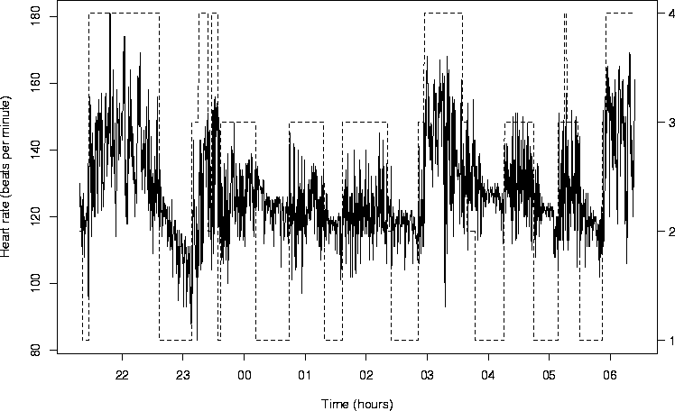
BabyECG,
is a record of the infant's heart rate (in beats per minute).
BabySS is a record of the infant's sleep state on a scale
of 1 to 4 as determined by a trained expert monitoring EEG (brain)
and EOG (eye-movement). The sleep state codes are
1=quiet sleep, 2=between quiet and active sleep, 3=active sleep,
4=awake.
BabyECG time series is a nice example of a non-stationary
time series whose spectral (time-scale) properties vary over time.
The function ewspec can be used to anaylse
this time series to inspect the variation in the power of the
series over time and scales.
The BabySS time series is a useful independent time series
that can be associated with changing power in the BabyECG
series. See the discussion in Nason, von Sachs and Kroisandt.
Nason, G.P., von Sachs, R. and Kroisandt, G. (1998). Wavelet processes and adaptive estimation of the evolutionary wavelet spectrum. Technical Report, Department of Mathematics University of Bristol/ Fachbereich Mathematik, Kaiserslautern.
#
# Plot the BabyECG data with BabySS overlaid
#
# Note the following code does some clever scaling to get the two
# time series overlaid.
#
myhrs <- c(22, 23, 24, 25, 26, 27, 28, 29, 30)
mylab <- c("22", "23", "00", "01", "02", "03", "04", "05", "06")
initsecs <- 59 + 60 * (17 + 60 * 21)
mysecs <- (myhrs * 3600)
secsat <- (mysecs - initsecs)/16
mxy <- max(BabyECG)
mny <- min(BabyECG)
ro <- range(BabySS)
no <- ((mxy - mny) * (BabySS - ro[1]))/(ro[2] - ro[1]) + mny
rc <- 0:4
nc <- ((mxy - mny) * (rc - ro[1]))/(ro[2] - ro[1]) + mny
plot(1:length(BabyECG), BabyECG, xaxt = "n", type = "l", xlab =
	"Time (hours)", ylab = "Heart rate (beats per minute)")
lines(1:length(BabyECG), no, lty = 3)
axis(1, at = secsat, labels = mylab)
axis(4, at = nc, labels = as.character(rc))
#
# Sleep state is the right hand axis
#
#
