plot.wp

Plot wavelet packet transform coefficients.

DESCRIPTION

USAGE

plot.wp(wp, nvwp = NULL, main = "Wavelet Packet Decomposition", 
    sub, first.level = 5, scaling = "compensated", dotted.turn.on = 5, 
    color.force = F, WaveletColor = 2, NodeVecColor = 3, fast = F, 
    SmoothedLines = T, ...) 

REQUIRED ARGUMENTS

wp

The wp object whose coefficients you wish to plot.

OPTIONAL ARGUMENTS

nvwp

An optional associated wavelet packet node vector class object. This object is a list of packets in the wavelet packet table. If this argument is specified then it is possible to highlight the packets in the nvwp objects in a different color.

main

The main title of the plot.

sub

A subtitle for the plot.

first.level

The first resolution level to begin plotting at. This argument can be quite useful when you want to supress some of the coarser levels in the diagram.

scaling

How you want the coefficients to be scaled. The options are: global - one scale factor is chosen for the whole plot. The scale factor depends on the coefficient to be included on the plot that has the largest absolute value. The global option is useful when comparing coefficients that might appear anywhere in the plot; by.level - a scale factor is chosen for each resolution level in the plot. The scale factor for a level depends on the coefficient in that level that has the largest absolute value. The by.level option is useful when you wish to compare coefficients within a resolution level.

The other option is compensated which is the same as global except for that finer scales' coefficients are scaled up by a factor of SQRT(2) for compensated.

I don't know why compensated is the default option?

dotted.turn.on

The plot usually includes some dotted vertical bars that separate wavelet packets to make it clearer which packets are which. This option controls the coarsest resolution level at which dotted lines appear. All levels equal to and finer than this level will receive the vertical dotted lines.

color.force

If F then some "clever" code in CanUseMoreThanOneColor tries to figure out how many colours can be used and hence whether colour can be used to pick out wavelet packets or elements of a node vector. This option was designed to work with S. It probably doesn't work too well with R and so it is probably best to set color.force=T. In this way no interrogation is done and the lines/packets are plotted in the appropriate colours with no questions asked.

WaveletColor

A colour specification for the colour for wavelet coefficients. Wavelet coefficients are a component of wavelet packet coefficients and this option allows them to be drawn in a different color. In S use an integer to select a color (from the colour table). If you use 1 you'll use the same colour as the plot axis etc. Higher values will give you different colours. In R you can use names like "red", "blue" to select the colors. In R you'll also need to set the color.force option to T.

NodeVecColor

If a nvwp object is supplied this option can force coefficients that are part of that nvwp to be drawn in the specified color. See the explanation for the WaveletColor option above about specification in S and R.

fast

This option no longer does anything.

SmoothedLines

If T then the scaling function coefficients are drawn using lines (and look like mini versions of the original). If F then the scaling function coefficients are drawn using segments and look like a coarser shadowy version of the original.

VALUE

SIDE EFFECTS

DETAILS

Given a wavelet packet object wp it possesses nlevels(wp) resolution levels. In WaveThresh the coarsest level is level 0 and the finest is level nlevels-1. For wavelet packets the number of packets at level j is 2^(nlevels-j).

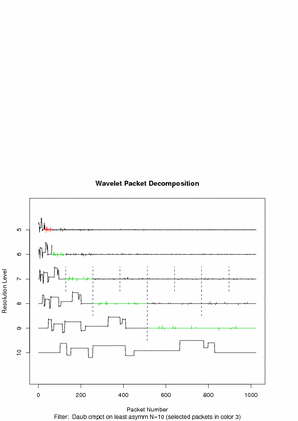
This function plots the wavelet packet coefficients. At the bottom of the plot the original input function (if present) is plotted. Then levels above the original plot successively coarser wavelet packet coefficients. From the Mallat transform point of view smoothing goes up off the the left of the picture and detail to the right. The packets are indexed from 0 to the number of packets going from left to right within each resolution level.

The function has the ability to draw wavelet coefficients in a different color using the WaveletColor argument.

Optionally, if a node vector wavelet packet object is also supplied then packets in that node vector can be highlighted in a another colour determined by the NodeVecColor.

Packets are drawn on the plot and can be separated by vertical dotted lines. The resolution levels at which this happens can be controlled by the dotted.turn.on option. The coarsest resolution level to be drawn is controlled by the first.level option.

RELEASE

SEE ALSO

EXAMPLES

#
# Generate some test data
#
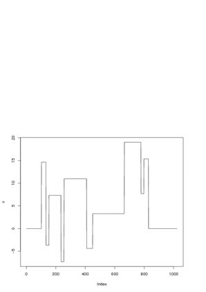
v <- DJ.EX()$blocks
#
# Let's plot these to see what they look like
#
plot(v, type="l")

#
# Do a wavelet packet transform
#
vwp <- wp(v)
#
# And create a node vector
#
vnv <- MaNoVe(vwp)
#
# Now plot the wavelet packets with the associated node vector
#
plot(vwp, vnv, color.force=T, WaveletColor="red", dotted.turn.on=7)

#
# The wavelet coefficients are plotted in red. Packets from the node vector
# are depicted in green. The node vector gets plotted after the wavelet
# coefficients so the green packets overlay the red (retry the plot command
# but without the vnv object to see just the
# wavelet coefficients). The vertical dotted lines start at resolution
# level 7.
#
#