WaveThresh
Help
PsiJ
Compute discrete autocorrelation wavelets.
DESCRIPTION
This function computes discrete autocorrelation wavelets.
The inner products of the discrete autocorrelation wavelets
are computed by the routine ipndacw.
USAGE
PsiJ(J, filter.number = 10, family = "DaubLeAsymm", tol = 1e-100, OPLENGTH=2000)
REQUIRED ARGUMENTS
- J
- Discrete autocorrelation wavelets will be computed for scales -1 up to
scale J. This number should be a negative integer.
OPTIONAL ARGUMENTS
- filter.number
- The index of the wavelet used to compute the discrete autocorrelation
wavelets.
- family
- The family of wavelet used to compute the discrete autocorrelation
wavelets.
- tol
- In the brute force computation for Daubechies compactly supported
wavelets many inner product computations are performed. This tolerance
discounts any results which are smaller than
tol which
effectively defines how long the inner product/autocorrelation products
are.
- OPLENGTH
- This integer variable defines some workspace of length OPLENGTH.
The code uses this workspace. If the workspace is not long
enough then the routine will stop and probably tell you what
OPLENGTH should be set to.
VALUE
A list containing -J components, numbered from 1 to -J. The [[j]]th
component contains the discrete autocorrelation wavelet at
scale j.
SIDE EFFECTS
None
DETAILS
This function computes the discrete autocorrelation wavelets.
It does not have any direct use for time-scale analysis
(e.g. ewspec). However, it is useful
to be able to numerically compute the discrete autocorrelation
wavelets for arbitrary wavelets and scales as there are still
unanswered theoretical questions concerning the wavelets.
The method is a brute force -- a more elegant solution would
probably be based on interpolatory schemes.
Horizontal scale. This routine returns only
the values of the discrete autocorrelation wavelets and not their
horiztonal positions. Each discrete autocorrelation wavelet
is compactly supported with the support determined from the
compactly supported wavelet that generates it. See
the paper by Nason, von Sachs and Kroisandt which defines the horiztonal
scale (but basically the finer scale discrete autocorrelation wavelets
are interpolated versions of the coarser ones. When one goes from scale
j to j-1 (negative j remember) an extra point is inserted between all
of the old points and the discrete autocorrelation wavelet value is
computed there. Thus as J tends to negative infinity the numerical
approximation tends towards the continuous autocorrelation wavelet.
This function stores any discrete autocorrelation wavelet sets that
it computes. The storage mechanism is not as advanced as that for
ipndacw and its subsidiary routines
rmget and firstdot
but helps a little bit. The Psiname function
defines the naming convention for objects returned by this function.
Sometimes it is useful to have the discrete autocorrelation wavelets
stored in matrix form. The PsiJmat does this.
RELEASE
Version 3.9 Copyright Guy Nason 1998
REFERENCES
Nason, G.P., von Sachs, R. and Kroisandt, G. (1998).
Wavelet processes and adaptive estimation of the evolutionary wavelet
spectrum. Technical Report, Department of Mathematics University of
Bristol/ Fachbereich Mathematik, Kaiserslautern.
SEE ALSO
ewspec,
ipndacw,
PsiJmat,
Psiname.
EXAMPLES
#
# Let us create the discrete autocorrelation wavelets for the Haar wavelet.
# We shall create up to scale 4.
#
> PsiJ(-4, filter.number=1, family="DaubExPhase")
Computing PsiJ
Returning precomputed version
Took 0.00999999 seconds
[[1]]:
[1] -0.5 1.0 -0.5
[[2]]:
[1] -0.25 -0.50 0.25 1.00 0.25 -0.50 -0.25
[[3]]:
[1] -0.125 -0.250 -0.375 -0.500 -0.125 0.250 0.625 1.000 0.625 0.250
[11] -0.125 -0.500 -0.375 -0.250 -0.125
[[4]]:
[1] -0.0625 -0.1250 -0.1875 -0.2500 -0.3125 -0.3750 -0.4375 -0.5000 -0.3125
[10] -0.1250 0.0625 0.2500 0.4375 0.6250 0.8125 1.0000 0.8125 0.6250
[19] 0.4375 0.2500 0.0625 -0.1250 -0.3125 -0.5000 -0.4375 -0.3750 -0.3125
[28] -0.2500 -0.1875 -0.1250 -0.0625
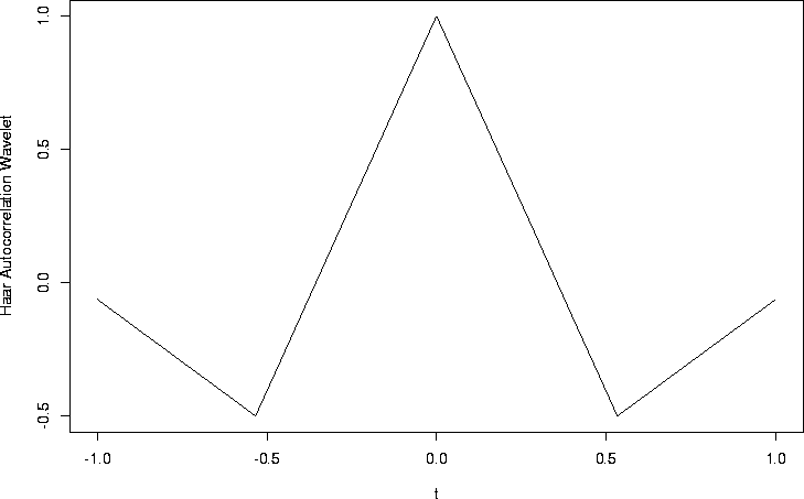
#
# You can plot the fourth component to get an idea of what the
# autocorrelation wavelet looks like.
#
# Note that the previous call stores the autocorrelation wavelet
# in Psi.4.1.DaubExPhase. This is mainly so that it doesn't have to
# be recomputed.
#
# Note that the x-coordinates in the following are approximate.
#
> plot(seq(from=-1, to=1, length=length(Psi.4.1.DaubExPhase[[4]])),
+ Psi.4.1.DaubExPhase[[4]], type="l",
+ xlab = "t", ylab = "Haar Autocorrelation Wavelet")
 #
# Now let us repeat the above for the Daubechies Least-Asymmetric wavelet
# with 10 vanishing moments.
# We shall create up to scale 6, a higher resolution version than last
# time.
#
> PsiJ(-6, filter.number=10, family="DaubLeAsymm")
[[1]]:
[1] 3.537571e-07 5.699601e-16 -7.512135e-06 -7.705013e-15 7.662378e-05
[6] 5.637163e-14 -5.010016e-04 -2.419432e-13 2.368371e-03 9.976593e-13
[11] -8.684028e-03 -1.945435e-12 2.605208e-02 6.245832e-12 -6.773542e-02
[16] 4.704777e-12 1.693386e-01 2.011086e-10 -6.209080e-01 1.000000e+00
[21] -6.209080e-01 2.011086e-10 1.693386e-01 4.704777e-12 -6.773542e-02
[26] 6.245832e-12 2.605208e-02 -1.945435e-12 -8.684028e-03 9.976593e-13
[31] 2.368371e-03 -2.419432e-13 -5.010016e-04 5.637163e-14 7.662378e-05
[36] -7.705013e-15 -7.512135e-06 5.699601e-16 3.537571e-07
[[2]]
scale 2 etc. etc.
[[3]] scale 3 etc. etc.
scales [[4]] and [[5]]...
[[6]]
...
remaining scale 6 elements...
...
[2371] -1.472225e-31 -1.176478e-31 -4.069848e-32 -2.932736e-41 6.855259e-33
[2376] 5.540202e-33 2.286296e-33 1.164962e-42 -3.134088e-35 3.427783e-44
[2381] -1.442993e-34 -2.480298e-44 5.325726e-35 9.346398e-45 -2.699644e-36
[2386] -4.878634e-46 -4.489527e-36 -4.339365e-46 1.891864e-36 2.452556e-46
[2391] -3.828924e-37 -4.268733e-47 4.161874e-38 3.157694e-48 -1.959885e-39
#
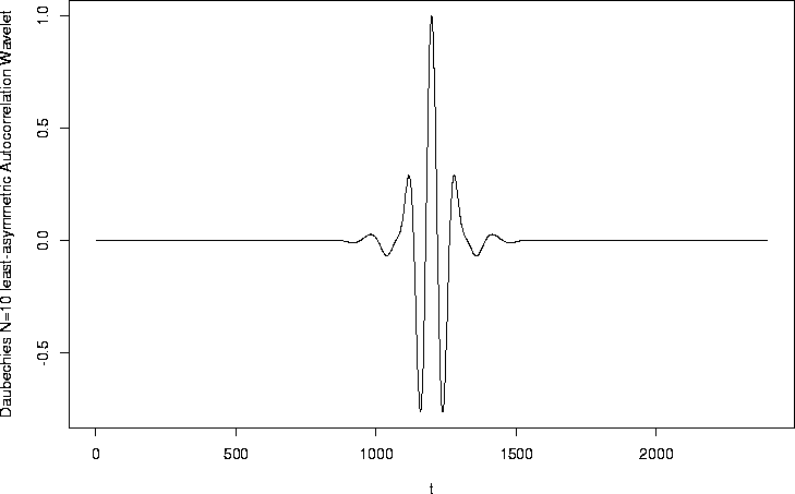
# Let's now plot the 6th component (6th scale, this is the finest
# resolution, all the other scales will be coarser representations)
#
# Note that the previous call stores the autocorrelation wavelet
# in Psi.6.10.DaubLeAsymm.
#
# Note that the x-coordinates in the following are non-existant!
#
> tsplot(Psi.6.10.DaubExPhase[[6]], xlab = "t",
+ ylab = "Daubechies N=10 least-asymmetric Autocorrelation Wavelet")
#
# Now let us repeat the above for the Daubechies Least-Asymmetric wavelet
# with 10 vanishing moments.
# We shall create up to scale 6, a higher resolution version than last
# time.
#
> PsiJ(-6, filter.number=10, family="DaubLeAsymm")
[[1]]:
[1] 3.537571e-07 5.699601e-16 -7.512135e-06 -7.705013e-15 7.662378e-05
[6] 5.637163e-14 -5.010016e-04 -2.419432e-13 2.368371e-03 9.976593e-13
[11] -8.684028e-03 -1.945435e-12 2.605208e-02 6.245832e-12 -6.773542e-02
[16] 4.704777e-12 1.693386e-01 2.011086e-10 -6.209080e-01 1.000000e+00
[21] -6.209080e-01 2.011086e-10 1.693386e-01 4.704777e-12 -6.773542e-02
[26] 6.245832e-12 2.605208e-02 -1.945435e-12 -8.684028e-03 9.976593e-13
[31] 2.368371e-03 -2.419432e-13 -5.010016e-04 5.637163e-14 7.662378e-05
[36] -7.705013e-15 -7.512135e-06 5.699601e-16 3.537571e-07
[[2]]
scale 2 etc. etc.
[[3]] scale 3 etc. etc.
scales [[4]] and [[5]]...
[[6]]
...
remaining scale 6 elements...
...
[2371] -1.472225e-31 -1.176478e-31 -4.069848e-32 -2.932736e-41 6.855259e-33
[2376] 5.540202e-33 2.286296e-33 1.164962e-42 -3.134088e-35 3.427783e-44
[2381] -1.442993e-34 -2.480298e-44 5.325726e-35 9.346398e-45 -2.699644e-36
[2386] -4.878634e-46 -4.489527e-36 -4.339365e-46 1.891864e-36 2.452556e-46
[2391] -3.828924e-37 -4.268733e-47 4.161874e-38 3.157694e-48 -1.959885e-39
#
# Let's now plot the 6th component (6th scale, this is the finest
# resolution, all the other scales will be coarser representations)
#
# Note that the previous call stores the autocorrelation wavelet
# in Psi.6.10.DaubLeAsymm.
#
# Note that the x-coordinates in the following are non-existant!
#
> tsplot(Psi.6.10.DaubExPhase[[6]], xlab = "t",
+ ylab = "Daubechies N=10 least-asymmetric Autocorrelation Wavelet")