WaveThresh Help

BAYES.THR

Bayesian wavelet thresholding.

DESCRIPTION

This function carries out Bayesian wavelet thresholding of noisy data, using the BayesThresh method of Abramovich, Sapatinas, & Silverman (1998).

USAGE

BAYES.THR(data, alpha = 0.5, beta = 1, filter.number = 8, family =
"DaubLeAsymm", bc = "periodic", dev = var, j0 = 5, plotfn = F)

REQUIRED ARGUMENTS

data: A vector of length a power of two, containing noisy data to be thresholded.

OPTIONAL ARGUMENTS

alpha, beta: Hyperparameters which determine the priors placed on the wavelet coefficients. Both alpha and beta take positive values; see Abramovich, Sapatinas, & Silverman (1998) or Chipman & Wolfson (1999) for more details on selecting alpha and beta.
filter.number: This selects the smoothness of wavelet that you want to use in the decomposition. By default this is 10, the Daubechies least-asymmetric orthonormal compactly supported wavelet with 10 vanishing moments.
For the ``wavelets on the interval'' (bc="interval") transform the filter number ranges from 1 to 8. See the table of filter coefficients indexed after the reference to Cohen, Daubechies and Vial, (1993).
family: Specifies the family of wavelets that you want to use. Two popular options are "DaubExPhase" and "DaubLeAsymm" but see the help for filter.select for more possibilities.
This argument is ignored for the ``wavelets on the interval'' transform (bc="interval").
bc: Specifies the boundary handling. If bc="periodic" the default, then the function you decompose is assumed to be periodic on it's interval of definition, if bc="symmetric" then the function beyond its boundaries is assumed to be a symmetric reflection of the function in the boundary. The symmetric option was the implicit default in releases prior to 2.2. If bc=="interval" then the ``wavelets on the interval algorithm'' due to Cohen, Daubechies and Vial is used. (The WaveThresh implementation of the ``wavelets on the interval transform'' was coded by Piotr Fryzlewicz, Department of Mathematics, Wroclaw University of Technology, Poland; this code was largely based on code written by Markus Monnerjahn, RHRK, Universitat Kaiserslautern; integration into WaveThresh by GPN).
dev: This argument supplies the function to be used to compute the spread of the absolute values coefficients. The function supplied must return a value of spread on the variance scale (i.e. not standard deviation) such as the var() function. A popular, useful and robust alternative is the madmad function.
j0: The primary resolution level. While BayesThresh thresholds at all resolution levels, j0 is used in assessing the universal threshold which is used in the empirical Bayes estimation of hyperparameters.
plotfn: If TRUE, BAYES.THR draws the noisy data and the thresholded function estimate.

VALUE

A vector containing the thresholded estimate of the function from which the data was drawn.

SIDE EFFECTS

If plotfn = TRUE, the noisy data and function estimate are plotted.

DETAILS

A mixture prior consisting of a zero-mean normal distribution and a point mass at zero is placed on each wavelet coefficient. The empirical coefficients are then calculated and the priors updated to give posterior distributions for each coefficient. The thresholded value of each coefficient is the median of that coefficient's posterior distribution. See Abramovich, Sapatinas, & Silverman (1998) for more details of the procedure; the help page for threshold.wd has more information about wavelet thresholding in general.

The function wave.band uses the same priors to compute posterior credible intervals for the regression function, using the method described by Barber, Nason, & Silverman (2001).

RELEASE

3.9.5
Code by Fanis Sapatinas/Felix Abramovich
Documentation by Stuart Barber

EXAMPLES

#
# Generate some noisy test data and plot it.
#
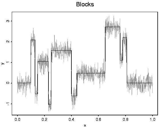
blocks.data <- test.data(type="blocks", rsnr=4, n=1024, plotfn=T) 

 

#
# Now try BAYES.THR with the default parameters.
#
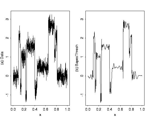
blocks.thr <- BAYES.THR(blocks.data$ynoise, plotfn=T)) 

 

#
# The default wavelet is Daubechies' least asymmetric wavelet 
# with 8 vanishing moments; quite a smooth wavelet. Since the 
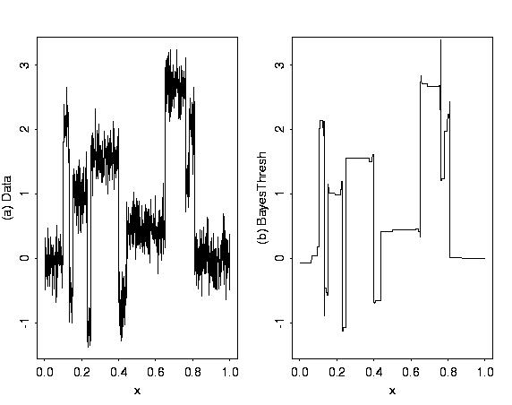
# flat sections are still rather noisy, try Haar wavelets:
# 
blocks.thr <- BAYES.THR(blocks.data$ynoise, plotfn=T, filter.number=1,
        family = "DaubExPhase")) 

 

#
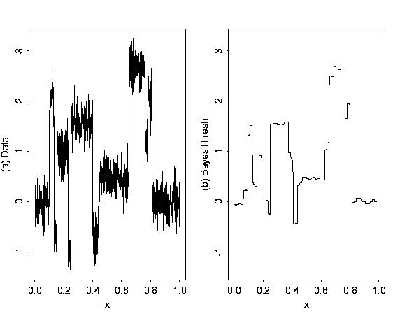
# To show the importance of a sensible prior, consider alpha = 4, 
# beta = 1 (which implies a smoother prior than the default). 
#
blocks.thr <- BAYES.THR(blocks.data$ynoise, plotfn=T, filter.number=1,
        family = "DaubExPhase", alpha=4, beta=1)) 

 

#
# Here, the extreme values of the function are being smoothed towards zero.
#