WaveThresh Help

makegrid

Interpolate data to a grid.

DESCRIPTION

This function takes a set of univariate (x,y) data with x arbitrary in (0,1) and linearly interpolates (x,y) to an equally spaced dyadic grid.

USAGE

makegrid(t, y, gridn = 2^(floor(log(length(t)-1,2)) + 1))

REQUIRED ARGUMENTS

t: A vector of x data. Each of the entries of x must lie between 0 and 1.
y: A vector of y data. Each entry of y corresponds to the same-positioned entry in x and so y must be of the same length as x.

OPTIONAL ARGUMENTS

gridn: The number of grid points in the dyadic grid that the (x,y) gets interpolated to. By default this is the next power of two larger than the length of x.

VALUE

An object of class griddata.

SIDE EFFECTS

None

DETAILS

One method for performing wavelet regression on data that is not equally spaced nor of power of two length is that described in Kovac, (1997) and Kovac and Silverman, (2000).

The Kovac-Silverman algorithm linearly interpolates arbitrarily spaced (x,y) data to a dyadic grid and applies wavelet shrinkage to the interpolated data. However, if one assumes that the original data obeys a signal+noise model with iid data the interpolated data will be correlated due to the interpolation. This fact needs to be taken into account after taking the DWT and before thresholding one realizes that each coefficient has its own variance. The Kovac-Silverman algorithm computes this variance efficiently using knowledge of the interpolation scheme.

RELEASE

EXAMPLES

#
# Generate some values in (0,1), then sort them (for plotting)
#
tt <- sort(runif(100))
#
# Now evaluate the doppler function and add
# some noise.
#
yy <- doppler(tt) + rnorm(100, 0, 0.15)
#
# Now make the grid with this data
#
yygrid <- makegrid(t=tt, y=yy)
#
# Jolly good. Now let's take the wavelet transform of this gridded data.
# Note that we have to use the irregwd function
# of the gridded data as it computes the variances of the coefficients
# as well as the coefficients themselves.
#
yyirregwd <- irregwd(yygrid)
#
# You might want to plot the coefficients
#
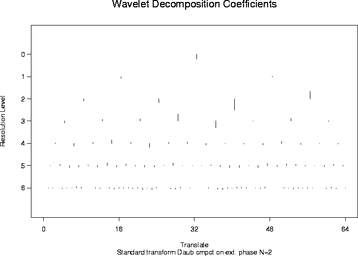
# If you want to see the actual coefficients you have to first convert
# the class of the yyirregwd object to a wd object and then use
# plot.wd like this
#
yyirregwd2 <- yyirregwd
class(yyirregwd2) <- "wd"
plot(yyirregwd2)

#
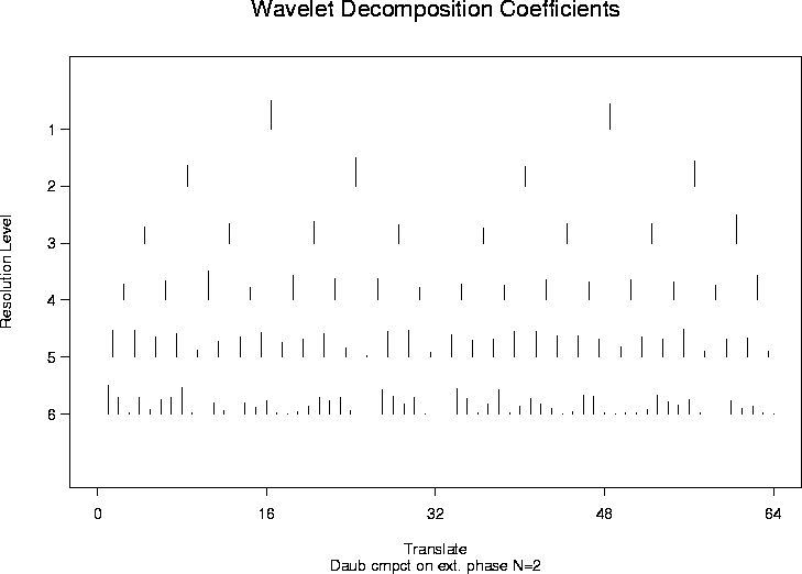
# If you want to see the variance factors (essentially the coefficient
# variances divided by the overall variance). Then just use
# plot.irregwd
#
plot(yyirregwd)

#
# Ok. So you've seen the coefficients. Now let's do some thresholding.
#
yy.thresh.sure <- threshold(yyirregwd, policy="sure", type="soft", dev=madmad)
#
# And now do the reconstruct
#
yy.wr <- wr(yy.thresh.sure)
#
# And you can even plot the answer on the new grid!
#
plot(yygrid$gridt, yy.wr, type="l")
#
# And superimpose the original data!
#
points(tt, yy)

#
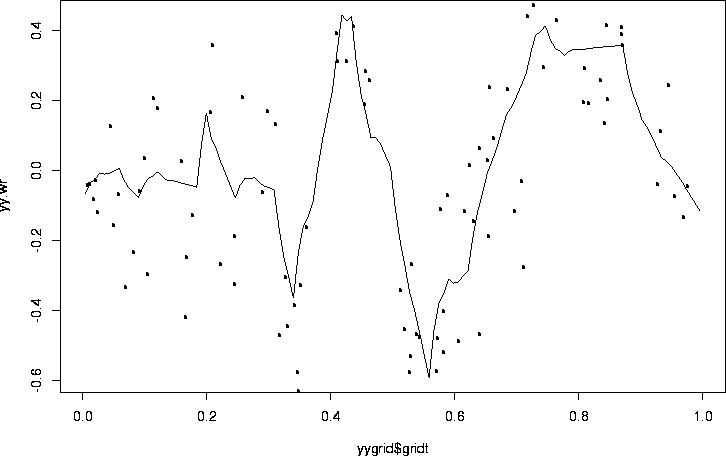# This is sort of Doppler like!