WaveThresh
Help
plot.wd
Plot wavelet transform coefficients.
DESCRIPTION
This function plots discrete wavelet transform coefficients arising from
a wd object.
USAGE
plot.wd(wd, xlabvals, first.level = 0,
	main = "Wavelet Decomposition Coefficients", scaling = "global",
	rhlab = F, sub, NotPlotVal = 0.005, xlab = "Translate",
	ylab = "Resolution Level",
	aspect = "Identity", ...)
REQUIRED ARGUMENTS
- wd
- The wd object whose coefficients you wish to
plot.
OPTIONAL ARGUMENTS
- xlabvals
- A vector containing the "true" x-axis numbers that went with the
vector that was transformed to produce the wd
object supplied as the first argument to this function. If this argument
is missing then the function tries to make up a sensible set of x-axis
labels.
- first.level
- The first resolution level to begin plotting at. This argument can
be quite useful when you want to supress some of the coarser levels
in the diagram.
- main
- The main title of the plot.
- scaling
- How you want the coefficients to be scaled. The options are:
global - one scale factor is chosen for the whole plot.
The scale factor depends on the coefficient to be included on the
plot that has the largest absolute value. The global
option is useful when comparing coefficients that might appear anywhere
in the plot; by.level - a scale factor is chosen for
each resolution level in the plot. The scale factor for a level
depends on the coefficient in that level that has the largest
absolute value. The by.level option is useful when
you wish to compare coefficients within a resolution level.
The two other options are compensated and
super which are the same as global except
for that finer scales' coefficients are scaled up by a factor
of SQRT(2) for compensated and 2 for super.
These latter two options are sometimes useful (more useful for
non-decimated wd objects, where they
act as a sort of ipndacw matrix operator).
- rhlab
- If
T then a set of labels is produced on the right hand
axis. The axis labels in this case refer to the scale factors used
to scale each level and correspond to value of the largest coefficient
(in absolute value) in each scale
(when scaling=="by.level")
or absolutely (when scaling="global").
If the rhlab argument is F then no right
hand axis labels are produced.
- sub
- A subtitle for the plot.
- NotPlotVal
- This argument ensures that if all (scaled) coefficients in a resolution
level are below
NotPlotVal in absolute value then the
whole resolution level is not plotted. This can be useful when plotting
a wd object that is sparse (or has been
thresholded and necessarily many coefficients might well be zero)
as it speeds up the plot because whole levels do not have to be
plotted (the function that does the plotting [segments()]
is quite a slow function). Note that the value of
NotPlotVal refers to scaled coefficients, those
that have been scaled by this function (on any resolution level
all coefficients are scaled to lie between -0.5 and 0.5).
- xlab
- A title for the x-axis
- ylab
- A title for the y-axis
- aspect
- This argument describes the name (as a character string) of a function
to be applied to the coefficients before plotting. By default the
argument is
"Identity", i.e. the coefficients are plotted
as is. This argument is most useful when a complex-valued
wavelets are plotted you could use "Mod" to plot the
modulus of the coefficients, or "Re" to plot the real
parts of the coefficients or "Arg" to plot the argument
of the coefficients. Also, the aspect argument can
be useful for the ordinary wavelet transforms as well if you are
interested in a particular transform of the coefficients.
VALUE
If rhlab==T then the scaling factors applied to each scale
level are returned. Otherwise NULL is returned.
SIDE EFFECTS
A plot of the coefficients contained within the wd
object is produced.
DETAILS
Produces a plot similar to the ones in
Donoho and Johnstone, 1994.
A wavelet decomposition of a signal consists of discrete wavelet
coefficients at different scales (resolution levels) and locations.
This function plots the coefficients as a pyramid (derived from
Mallat's pyramid algorithm).
See the examples below.
The resolution levels are stacked one above the other: coarse scale coefficients
are always towards the top of the plot, fine scale coefficients are always
located toward the bottom of the plot. The location of coefficients increases
from left to right across the plot in synchrony with the input signal to
the wd object. In other words the position of a
coefficient along a line is indicative of the associated wavelet basis
function's translate number.
The actual coefficients are plotted
using S-Plus's segments() function. This plots each coefficient
as a vertical line with positive coefficients being plotted above an imaginary
centre line and negative coefficients being plotted below.
The resolution levels are labelled on the left-hand side axis, and if
rhlab==T the maximum values of the absolute values of the
coefficients, for the particular level, are plotted on the right-hand axis.
The coefficients in the plot may be scaled in 4 ways. If you are interested
in comparing coefficients in different levels then the default scaling
option scaling=="global" is what you need. This works by
finding the coefficient with the largest absolute value amongst all
coeffients to be plotted and then scales all the other coefficients by
the largest so that all coefficients lie in the range -1/2 to 1/2. The
scaled coefficients are then plotted. If you are not interested in comparing
relative resolution levels and want to see all that goes on within a particular
scale then you should use the scaling option scaling=="by.level"
which picks out the largest coefficient (in absolute value) from each
level and scales each level separately. The "compensated"
and super options are like the "global" option
except that finer levels are scaled up (as discussed in the arguments
list above): this can be useful when plotting non-decimated wavelet
transform coefficients as it emphasizes the higher frequencies.
RELEASE
Version 3.5.3 Copyright Guy Nason 1994
SEE ALSO
wd.
EXAMPLES
#
# Generate some test data
#
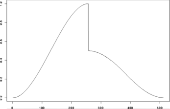
> test.data <- example.1()$y
> tsplot(test.data)
 #
# Decompose test.data and plot the wavelet coefficients
#
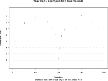
> wds <- wd(test.data)
> plot(wds)
#
# Decompose test.data and plot the wavelet coefficients
#
> wds <- wd(test.data)
> plot(wds)
 #
# Now do the time-ordered non-decimated wavelet transform of the same thing
#
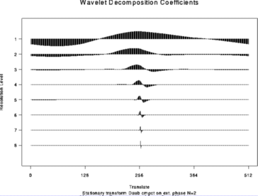
> wdS <- wd(test.data, type="station")
> plot(wdS)
#
# Now do the time-ordered non-decimated wavelet transform of the same thing
#
> wdS <- wd(test.data, type="station")
> plot(wdS)
 #
# Next example
# ------------
# The chirp signal is also another good example to use.
#
# Generate some test data
#
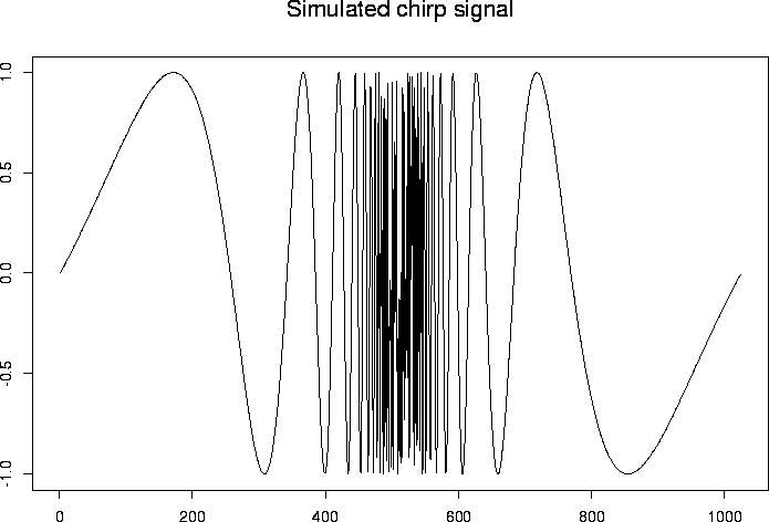
> test.chirp <- simchirp()$y
> tsplot(test.chirp, main="Simulated chirp signal")
#
# Next example
# ------------
# The chirp signal is also another good example to use.
#
# Generate some test data
#
> test.chirp <- simchirp()$y
> tsplot(test.chirp, main="Simulated chirp signal")
 #
# Now let's do the time-ordered non-decimated wavelet transform.
# For a change let's use Daubechies least-asymmetric phase wavelet with 8
# vanishing moments (a totally arbitrary choice, please don't read
# anything into it).
#
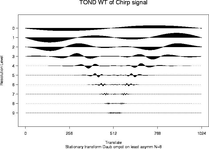
> chirpwdS <- wd(test.chirp, filter.number=8, family="DaubLeAsymm", type="station")
> plot(chirpwdS, main="TOND WT of Chirp signal")
#
# Now let's do the time-ordered non-decimated wavelet transform.
# For a change let's use Daubechies least-asymmetric phase wavelet with 8
# vanishing moments (a totally arbitrary choice, please don't read
# anything into it).
#
> chirpwdS <- wd(test.chirp, filter.number=8, family="DaubLeAsymm", type="station")
> plot(chirpwdS, main="TOND WT of Chirp signal")

 #
# Decompose test.data and plot the wavelet coefficients
#
> wds <- wd(test.data)
> plot(wds)
#
# Decompose test.data and plot the wavelet coefficients
#
> wds <- wd(test.data)
> plot(wds)
 #
# Now do the time-ordered non-decimated wavelet transform of the same thing
#
> wdS <- wd(test.data, type="station")
> plot(wdS)
#
# Now do the time-ordered non-decimated wavelet transform of the same thing
#
> wdS <- wd(test.data, type="station")
> plot(wdS)
 #
# Next example
# ------------
# The chirp signal is also another good example to use.
#
# Generate some test data
#
> test.chirp <- simchirp()$y
> tsplot(test.chirp, main="Simulated chirp signal")
#
# Next example
# ------------
# The chirp signal is also another good example to use.
#
# Generate some test data
#
> test.chirp <- simchirp()$y
> tsplot(test.chirp, main="Simulated chirp signal")
 #
# Now let's do the time-ordered non-decimated wavelet transform.
# For a change let's use Daubechies least-asymmetric phase wavelet with 8
# vanishing moments (a totally arbitrary choice, please don't read
# anything into it).
#
> chirpwdS <- wd(test.chirp, filter.number=8, family="DaubLeAsymm", type="station")
> plot(chirpwdS, main="TOND WT of Chirp signal")
#
# Now let's do the time-ordered non-decimated wavelet transform.
# For a change let's use Daubechies least-asymmetric phase wavelet with 8
# vanishing moments (a totally arbitrary choice, please don't read
# anything into it).
#
> chirpwdS <- wd(test.chirp, filter.number=8, family="DaubLeAsymm", type="station")
> plot(chirpwdS, main="TOND WT of Chirp signal")
