WaveThresh
Help
wd
Wavelet transform (decomposition).
DESCRIPTION
This function can perform two types of discrete wavelet
transform (DWT). The standard DWT computes the DWT
according to Mallat's pyramidal algorithm
(Mallat, 1989) (it also has the
ability to compute the wavelets on the interval transform
of Cohen, Daubechies and Vial, 1993).
The non-decimated DWT (NDWT) contains all possible shifted versions
of the DWT. The order of computation of the DWT is O(n), and
it is O(n log n) for the NDWT if n is the number of data points.
USAGE
wd(data, filter.number=10, family="DaubLeAsymm", type="wavelet",
bc="periodic", verbose=F, min.scale=0, precond=T)
REQUIRED ARGUMENTS
- data
- A vector containing the data you wish to decompose. The
length of this vector must be a power of 2.
OPTIONAL ARGUMENTS
- filter.number
- This selects the smoothness of wavelet that you
want to use in the decomposition. By default this is 10,
the Daubechies least-asymmetric orthonormal compactly supported wavelet
with 10 vanishing moments.
For the ``wavelets on the interval'' (bc="interval")
transform the filter number ranges from
1 to 8. See the table of filter coefficients indexed after the reference to
Cohen, Daubechies and Vial, 1993.
- family
- specifies the family of wavelets that you want to use.
Two popular options are "DaubExPhase" and "DaubLeAsymm" but see the
help for filter.select for more possibilities.
This argument is ignored for the ``wavelets on the interval'' transform
(bc="interval").
- type
- specifies the type of wavelet transform. This can be
"wavelet" (default) in which case the standard DWT is
performed (as in previous releases of WaveThresh). If type
is "station" then the non-decimated DWT is performed. At
present, only periodic boundary conditions can be used
with the non-decimated wavelet transform.
- bc
- specifies the boundary handling. If
bc="periodic" the
default, then the function you decompose is assumed to be
periodic on it's interval of definition, if
bc="symmetric" then the function beyond its boundaries is
assumed to be a symmetric reflection of the function in
the boundary. The symmetric option was the implicit
default in releases prior to 2.2. If bc=="interval" then
the ``wavelets on the interval algorithm'' due to
Cohen, Daubechies and Vial is used.
(The WaveThresh
implementation of the ``wavelets on the interval transform'' was
coded by Piotr Fryzlewicz,
Department of Mathematics,
Wroclaw University of Technology,
Poland; this code was largely based
on code written by
Markus Monnerjahn,
RHRK,
Universitat Kaiserslautern;
integration into WaveThresh by
GPN.
See the nice project report by
Piotr on this piece of code).
- verbose
- Controls the printing of "informative" messages
whilst the computations progress. Such messages are
generally annoying so it is turned off by default.
- min.scale
- Only used for the ``wavelets on the interval transform''. The wavelet
algorithm starts with fine scale data and iteratively coarsens it.
This argument controls how many times this iterative procedure
is applied by specifying at which scale level to stop decomposiing.
- precond
- Only used for the ``wavelets on the interval transform''. This
argument specifies whether preconditioning is applied (called
prefiltering in Cohen, Daubechies
and Vial, 1993. Preconditioning ensures that sequences
like 1,1,1,1 or 1,2,3,4 map to zero high pass coefficients.
VALUE
An object of class wd.
For boundary conditions apart from bc="interval"
this object is a list with the following components.
- C
- Vector of sets of successively smoothed data. The pyramid
structure of Mallat is stacked so that it fits into a
vector. The function accessC
should be used to extract a
set for a particular level.
- D
- Vector of sets of wavelet coefficients at different
resolution levels. Again, Mallat's
pyramid structure is
stacked into a vector. The function accessD
should be used to extract the coefficients for a particular
resolution level.
- nlevels
- The number of resolution levels. This depends on the
length of the data vector. If length(data)=2^m, then there
will be m resolution levels. This means there will be m
levels of wavelet coefficients (indexed 0,1,2,...,(m-1)),
and m+1 levels of smoothed data (indexed 0,1,2,...,m).
- fl.dbase
- There is more information stored in the C and D than
is described above. In the decomposition ``extra''
coefficients are generated that help take care of the
boundary effects, this database lists where these start
and finish, so the "true" data can be extracted.
- filter
- A list containing information about the filter
type: Contains the string "wavelet" or "station" depending on
which type of transform was performed.
- date
- The date the transform was performed.
- bc
- How the boundaries were handled.
If the ``wavelets on the interval'' transform is used (i.e.
bc="interval") then the internal structure of the wd
object is changed as follows.
SIDE EFFECTS
None
DETAILS
If type=="wavelet" then the code implements Mallat's
pyramid algorithm (Mallat 1989).
For more details of this implementation
see Nason and Silverman, 1994.
Essentially it works
like this: you start off with some data cm, which is a
real vector of length 2^m, say.
Then from this you obtain two vectors of length 2^(m-1).
One of these is a set of smoothed data, c(m-1), say. This
looks like a smoothed version of cm. The other is a
vector, d(m-1), say. This corresponds to the detail
removed in smoothing cm to c(m-1). More precisely, they
are the coefficients of the wavelet expansion
corresponding to the highest resolution wavelets in the
expansion. Similarly, c(m-2) and d(m-2) are obtained from
c(m-1), etc. until you reach c0 and d0.
All levels of smoothed data are stacked into a single
vector for memory efficiency and ease of transport across
the SPlus-C interface.
The smoothing is performed directly by convolution with
the wavelet filter (filter.select(n)$H, essentially low-
pass filtering), and then dyadic decimation (selecting
every other datum, see
Vaidyanathan (1990)). The detail
extraction is performed by the mirror filter of H, which
we call G and is a bandpass filter. G and H are also
known quadrature mirror filters.
There are now two methods of handling "boundary problems".
If you know that your function is periodic (on it's
interval) then use the bc="periodic" option, if you think
that the function is symmetric reflection about each
boundary then use bc="symmetric". You might also consider using
the "wavelets on the interval" transform which is suitable for data
arising from a function that is known to be defined on some compact
interval, see Cohen, Daubechies,
and Vial, 1993.
If you don't know then
it is wise to experiment with both methods, in any case,
if you don't have very much data don't infer too much
about your decomposition! If you have loads of data then
don't infer too much about the boundaries. It can be
easier to interpret the wavelet coefficients from a
bc="periodic" decomposition, so that is now the default.
Numerical Recipes implements some of the wavelets code, in
particular we have compared our code to "wt1" and "daub4"
on page 595. We are pleased to announce that our code
gives the same answers! The only difference that you
might notice is that one of the coefficients, at the
beginning or end of the decomposition, always appears in
the "wrong" place. This is not so, when you assume
periodic boundaries you can imagine the function defined
on a circle and you can basically place the coefficient at
the beginning or the end (because there is no beginning or
end, as it were).
The non-deciated DWT contains all circular shifts of the
standard DWT. Naively imagine that you do the standard
DWT on some data using the Haar wavelets. Coefficients 1
and 2 are added and difference, and also coefficients 3
and 4; 5 and 6 etc. If there is a discontinuity between 1
and 2 then you will pick it up within the transform. If it
is between 2 and 3 you will loose it. So it would be nice
to do the standard DWT using 2 and 3; 4 and 5 etc. In
other words, pick up the data and rotate it by one
position and you get another transform. You can do this in
one transform that also does more shifts at lower
resolution levels. There are a number of points to note
about this transform.
Note that a time-ordered non-decimated wavelet transform object
may be converted into a packet-ordered non-decimated wavelet
transform object (and vice versa)
by using the convert
function.
The NDWT is translation equivariant.
The DWT is neither translation invariant or equivariant.
The standard DWT is
orthogonal, the non-decimated transform is most definitely
not. This has the added disadvantage that non-decimated
wavelet coefficients, even if you supply independent normal noise.
This is unlike the standard DWT where the coefficients are
independent (normal noise).
RELEASE
Version 3.5.3 Copyright Guy Nason 1994
Integration of ``wavelets on the interval'' code by
Piotr Fryzlewicz and Markus Monnerjahn was
at Version 3.9.6, 1999.
SEE ALSO
wd.int,
wr,
wr.int,
wr.wd,
accessC,
accessD,
putD,
putC,
filter.select,
plot.wd,
threshold.
EXAMPLES
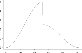
#
# Generate some test data
#
> test.data <- example.1()$y
> tsplot(test.data)
 #
# Decompose test.data and plot the wavelet coefficients
#
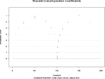
> wds <- wd(test.data)
> plot(wds)
#
# Decompose test.data and plot the wavelet coefficients
#
> wds <- wd(test.data)
> plot(wds)
 #
# Now do the time-ordered non-decimated wavelet transform of the same thing
#
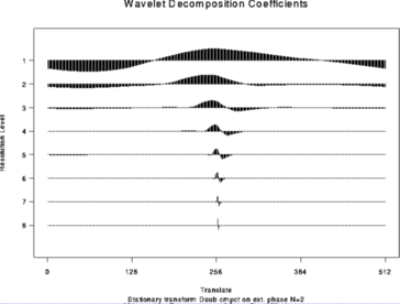
> wdS <- wd(test.data, type="station")
> plot(wdS)
#
# Now do the time-ordered non-decimated wavelet transform of the same thing
#
> wdS <- wd(test.data, type="station")
> plot(wdS)
 #
# Next example
# ------------
# The chirp signal is also another good example to use.
#
# Generate some test data
#
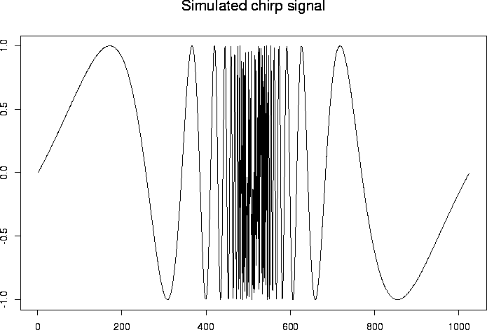
> test.chirp <- simchirp()$y
> tsplot(test.chirp, main="Simulated chirp signal")
#
# Next example
# ------------
# The chirp signal is also another good example to use.
#
# Generate some test data
#
> test.chirp <- simchirp()$y
> tsplot(test.chirp, main="Simulated chirp signal")
 #
# Now let's do the time-ordered non-decimated wavelet transform.
# For a change let's use Daubechies least-asymmetric phase wavelet with 8
# vanishing moments (a totally arbitrary choice, please don't read
# anything into it).
#
> chirpwdS <- wd(test.chirp, filter.number=8, family="DaubLeAsymm", type="station")
> plot(chirpwdS, main="TOND WT of Chirp signal")
#
# Now let's do the time-ordered non-decimated wavelet transform.
# For a change let's use Daubechies least-asymmetric phase wavelet with 8
# vanishing moments (a totally arbitrary choice, please don't read
# anything into it).
#
> chirpwdS <- wd(test.chirp, filter.number=8, family="DaubLeAsymm", type="station")
> plot(chirpwdS, main="TOND WT of Chirp signal")
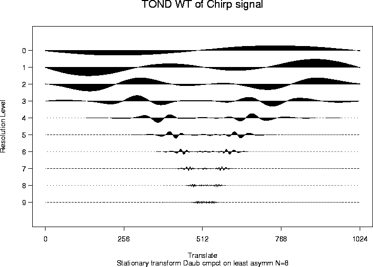 #
# Note that the coefficients in this plot are exactly the same as those
# generated by the packet-ordered non-decimated wavelet transform
# except that they are in a different order on each resolution level.
# See Nason, Sapatinas and Sawczenko, 1998
# for further information.
#
# Note that the coefficients in this plot are exactly the same as those
# generated by the packet-ordered non-decimated wavelet transform
# except that they are in a different order on each resolution level.
# See Nason, Sapatinas and Sawczenko, 1998
# for further information.