WaveThresh Help

wave.band

Posterior credible intervals for wavelet regression

DESCRIPTION

Computes posterior credible intervals for an unknown regression curve.

USAGE

function(data = 0, alpha = 0.5, beta = 1., filter.number = 8, family = 
        "DaubLeAsymm", bc = "periodic", dev = var, j0 = 3., plotfn = T, 
        retvalue = T, n = 128, type = "data", rsnr = 3)

REQUIRED ARGUMENTS

data: If type="data", then data should be a vector of data. The length of the vector should be a power of two not greater than 1024.
type: Either type="data", in which case a vector of data should be supplied, or type should specify a standard test function and wave.band will generate a test data set via a call to test.data. Permissible values for type are "blocks", "bumps", "doppler", "heavi", or "ppoly"; see the documentation for test.data for more details.

OPTIONAL ARGUMENTS

alpha, beta: Hyperparameters which determine the priors placed on the wavelet coefficients. Both alpha and beta take positive values; see Abramovich, Sapatinas, & Silverman (1998) or Chipman & Wolfson (1999) for more details on selecting alpha and beta.
filter.number: A parameter relating to the smoothness of wavelet that you want to use in the decomposition.
family: Specifies the family of wavelets to be used. Two popular options are "DaubExPhase" and "DaubLeAsymm" but see the help for filter.select for more possibilities.
bc: Specifies the boundary handling. If bc="periodic" the default, then the function you decompose is assumed to be periodic on it's interval of definition. Other boundary options exist, but are currently unsupported for this function.
dev: This argument supplies the function to be used to compute the spread of the absolute values coefficients. The function supplied must return a value of spread on the variance scale (i.e. not standard deviation) such as the var() function. A popular, useful and robust alternative is the madmad function.
j0: The primary resolution level; used in assessing the universal threshold which is used in the empirical Bayes estimation of hyperparameters.
plotfn: If plotfn=T, wave.band draws the noisy data, the BayesThresh function estimate, and pointwise 99 percent credible intervals for the regression function. If the value of type is not "data", then the true function will also be plotted.
retvalue: If retvalue=T, then a lengthy list of results will be returned. Note that if both plotfn and retvalue are set to F, then wave.band will return no results whatsoever.
n: If type is not "data", then a data vector of length n will be generated; note that n should be a power of two not greater than 1024.
rsnr: If type is not "data", then the data vector generated will have root signal-to-noise ratio as specified by rsnr.

VALUE

If retvalue=F, the value returned by wave.band is NULL. Otherwise, wave.band returns a list with the following components:

data: The data vector which has been analysed.
cumulants: A list containing four vectors named one, two, three, and four. Vector one contains the first cumulants of the regression function estimate, vector to the second cumulants and so on.
Kr.wd: A list of four wd objects. These contain the first to fourth cumulants of the wavelet coefficients, as well as recording the wavelet used in the decomposition.
bands: A list containing pointwise upper and lower credible limits for the regression function estimate for nominal coverage rates 80, 90, 95 and 99 percent. The widths of the credible intervals is also included. The vectors are named with "l", "u", and "w" indicating lower limits, upper limits, and intervals widths, while "80", "90", "95", and "99" refer to the nominal coverage rate.
param: A record of parameters in the call to wave.band.

SIDE EFFECTS

If plotfn=T, results are plotted on the current graphics device.

DETAILS

This function implements the WaveBand method of Barber, Nason, & Silverman (2001) to compute posterior credible intervals for a regression function. The credible intervals are found by approximating the posterior distribution of the estimated regression curve at each design point. A mixture prior with two components (a zero-mean normal and a point mass at zero) is placed on each wavelet coefficient and updated by the data to give the posteriors for the wavelet coefficients. This is the same prior used by Abramovich, Sapatinas, & Silverman (1998) in their BayesThresh method, implemented in the function BAYES.THR.

The cumulants of these posteriors are computed and stored in the wd objects returned by wave.band as Kr.wd. These are summed to give the posterior cumulants of the regression curve, which are used to fit a Johnson distribution (Johnson, 1949), using the algorithm of Hill, Hill, & Holder (1976). Percentage points of these distributions are computed by the algorithm of Hill (1976) and give the credible intervals themselves.

Code to implement the algorithms by Hill (1976) and Hill, Hill, & Holder (1976) were obtained from the StatLib archive.

RELEASE

3.9.7

EXAMPLES

#
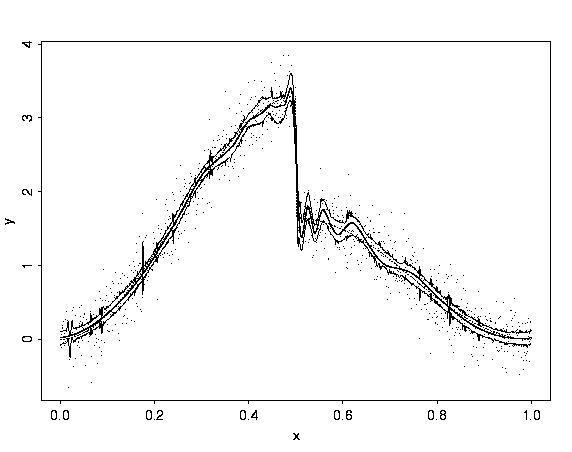
# First, look at the piecewise polynomial example.
#
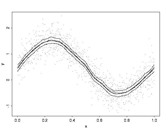
# This plot and the plots for the smooth example below show
# the data as points, the BayesThresh estimate (thick line), 
# pointwise 99 percent credible intervals (thin lines), and
# the true function (dotted thin line).
#
ppoly.wb <- wave.band(type = "ppoly", n = 1024, rsnr=4)

 


#
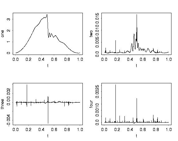
# Plotting the cumulants shows that there are significant 
# third and fourth cumulants in some places.
#
t <- (1:1024)/1024
plot(t, ppoly.wb$cumulants$one, type="l", xlab="t", ylab = "one")
plot(t, ppoly.wb$cumulants$two, type="l", xlab="t", ylab = "two")
plot(t, ppoly.wb$cumulants$three, type="l", xlab="t", ylab = "three")
plot(t, ppoly.wb$cumulants$four, type="l", xlab="t", ylab = "four")

 



#
# Now consider how much difference the prior can make.
# Consider a smooth example, first using the default prior,
# and then using a smoother prior.
#

gs <- sin(2*pi*t) + 2*(t - 0.5)^2
gs.noisy <- gs + rnorm(n=1024, sd=sqrt(var(gs))/2)
gs.wb1 <- wave.band(data=gs.noisy)

 


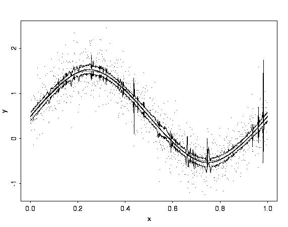
gs.wb2 <- wave.band(data=gs.noisy, alpha=4, beta=1)