WaveThresh
Help
plot.wst
Plot packet-ordered non-decimated wavelet transform coefficients.
DESCRIPTION
This function plots packet-ordered non-decimated wavelet packet transform
coefficients arising from
a wst object.
USAGE
plot.wst(wst, main = "Nondecimated Wavelet (Packet) Decomposition",
    sub, first.level = 5, scaling = "compensated", dotted.turn.on = 5,
    aspect = "Identity", ...)
REQUIRED ARGUMENTS
- wst
- The wst object whose coefficients you wish to
plot.
OPTIONAL ARGUMENTS
- main
- The main title of the plot.
- sub
- A subtitle for the plot.
- first.level
- The first resolution level to begin plotting at. This argument can
be quite useful when you want to supress some of the coarser levels
in the diagram.
- scaling
- How you want the coefficients to be scaled. The options are:
global - one scale factor is chosen for the whole plot.
The scale factor depends on the coefficient to be included on the
plot that has the largest absolute value. The global
option is useful when comparing coefficients that might appear anywhere
in the plot; by.level - a scale factor is chosen for
each resolution level in the plot. The scale factor for a level
depends on the coefficient in that level that has the largest
absolute value. The by.level option is useful when
you wish to compare coefficients within a resolution level.
The other option is compensated
which is the same as global except
for that finer scales' coefficients are scaled up by a factor
of SQRT(2) for compensated.
I don't know why compensated is the default option?
- dotted.turn.on
- The plot usually includes some dotted vertical bars that separate
wavelet packets to make it clearer which packets are which.
This option controls the coarsest resolution level at which dotted
lines appear. All levels equal to and finer than this level
will receive the vertical dotted lines.
- aspect
- A transform to apply to the coefficients before plotting. If the
coefficients are complex-valued and aspect="Identity" then
the modulus of the coefficients are plotted.
- ...
- Other arguments to plot
VALUE
Nothing.
SIDE EFFECTS
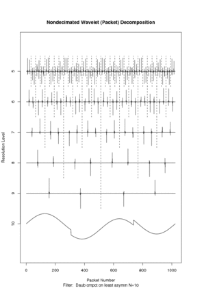
A plot of the packet ordered non-decimated wavelet packet coefficients
contained within the
wst object is produced.
DETAILS
A packet-ordered non-decimated wavelet packet object contains coefficients of
a signal (usually obtained by the wst packet-ordered
non-decimated wavelet packet transform).
Given a wavelet packet object wst it possesses
nlevels(wst)
resolution levels. In WaveThresh the coarsest level is level 0 and the
finest is level nlevels-1. For wavelet packets the number
of packets at level j is 2^(nlevels-j).
This function plots the coefficients. At the bottom of the
plot the original input function (if present) is plotted. Then
levels above the original plot successively coarser wavelet packet
coefficients. Each packet of coefficients is plotted within dotted
vertical lines. At the finest level there are two packets: one (the left
one) correspond to the wavelet coefficients that would be obtained using
the (standard) decimated wavelet transform function, wd,
and the other packet are those coefficients that would have been obtained
using the standard decimated wavelet transform after a unit cyclic shift.
For coarser levels there are more packets corresponding to different
cyclic shifts (although the computation is not performed using shifting
operations the effect is the same). For full details see
Nason and Silverman, 1995.
Packets are drawn on the plot and can be separated by vertical dotted lines.
The resolution levels at which this happens can be controlled by the
dotted.turn.on option. The coarsest resolution level to
be drawn is controlled by the first.level option.
RELEASE
Version 3.5.3 Copyright Guy Nason 1994
SEE ALSO
MaNoVe,
wst,
wst object,
EXAMPLES
#
# Generate some test data
#
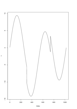
v <- DJ.EX()$heavi
#
# Let's plot these to see what they look like
#
plot(v, type="l")
 #
# Do a packet-ordered non-decimated wavelet packet transform
#
vwst <- wst(v)
#
# Now plot the coefficients
#
plot(vwst)
#
# Do a packet-ordered non-decimated wavelet packet transform
#
vwst <- wst(v)
#
# Now plot the coefficients
#
plot(vwst)
 #
# Note that the "original" function is at the bottom of the plot.
# The finest scale coefficients (two packets) are immediately above.
# Increasingly coarser scale coefficients are above that!
#
#
# Note that the "original" function is at the bottom of the plot.
# The finest scale coefficients (two packets) are immediately above.
# Increasingly coarser scale coefficients are above that!
#
 #
# Do a packet-ordered non-decimated wavelet packet transform
#
vwst <- wst(v)
#
# Now plot the coefficients
#
plot(vwst)
#
# Do a packet-ordered non-decimated wavelet packet transform
#
vwst <- wst(v)
#
# Now plot the coefficients
#
plot(vwst)
 #
# Note that the "original" function is at the bottom of the plot.
# The finest scale coefficients (two packets) are immediately above.
# Increasingly coarser scale coefficients are above that!
#
#
# Note that the "original" function is at the bottom of the plot.
# The finest scale coefficients (two packets) are immediately above.
# Increasingly coarser scale coefficients are above that!
#