WaveThresh
Help
wst
Packet-ordered non-decimated wavelet transform.
DESCRIPTION
Computes the packet-ordered non-decimated wavelet transform
(TI-transform). This algorithm is functionally equivalent to the
time-ordered non-decimated wavelet transform (computed by
wd with the type="station"
argument).
USAGE
wst(data, filter.number=10, family="DaubLeAsymm", verbose=F)
REQUIRED ARGUMENTS
- data
- A vector containing the data you wish to decompose. The
length of this vector must be a power of 2.
OPTIONAL ARGUMENTS
- filter.number
- This selects the smoothness of wavelet that you
want to use in the decomposition. By default this is 10,
the Daubechies least-asymmetric
orthonormal compactly supported wavelet with 10 vanishing moments.
- family
- specifies the family of wavelets that you want to use.
The options are "DaubExPhase" and "DaubLeAsymm".
- verbose
- Controls the printing of "informative" messages
whilst the computations progress. Such messages are
generally annoying so it is turned off by default.
VALUE
An object of class: wst.
The help for the wst describes the
intricate structure of this class of object.
SIDE EFFECTS
You may feel a little giddy.
DETAILS
The packet-ordered non-decimated wavelet transform is more properly known
as the TI-transform described by
Coifman and Donoho, 1995.
A description of this implementation can be found in
Nason and Silverman, 1995.
The coefficients produced by this transform are exactly the same
as those produced by the wd function with
the type="station" option except in that function
the coefficients are time-ordered. In the wst
function the coefficients are produced by a wavelet packet like
algorithm with a cyclic rotation step instead of processing with
the father wavelet mirror filter at each level.
The coefficients produced by this function are useful in curve estimation
problems in conjunction with the thresholding function
threshold.wst and either of the inversion functions
AvBasis.wst and
InvBasis.wst.
The coefficients produced by the time-ordered non-decimated
wavelet transform are more useful for time series applications: e.g.
the evolutionary wavelet spectrum computation performed by
ewspec.
Note that a time-ordered non-decimated wavelet transform object
may be converted into a packet-ordered non-decimated wavelet
transform object (and vice versa)
by using the convert
function.
RELEASE
Version 3.5.3 Copyright Guy Nason 1995
SEE ALSO
wst object,
threshold.wst,
AvBasis.wst,
InvBasis.wst,
filter.select,
convert,
ewspec,
plot.wst,
EXAMPLES
#
# Let's look at the packet-ordered non-decimated wavelet transform
# of the data we used to do the time-ordered non-decimated wavelet
# transform exhibited in the help page for wd.
#
> test.data <- example.1()$y
#
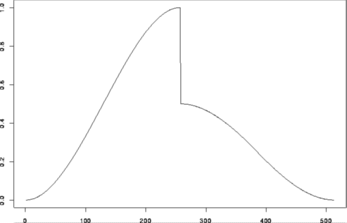
# Plot it to see what it looks like (piecewise polynomial)
#
> tsplot(test.data)
 #
# Now let's do the packet-ordered non-decimated wavelet transform.
#
> TDwst <- wst(test.data)
#
# And let's plot it....
#
> plot(TDwst)
#
# Now let's do the packet-ordered non-decimated wavelet transform.
#
> TDwst <- wst(test.data)
#
# And let's plot it....
#
> plot(TDwst)
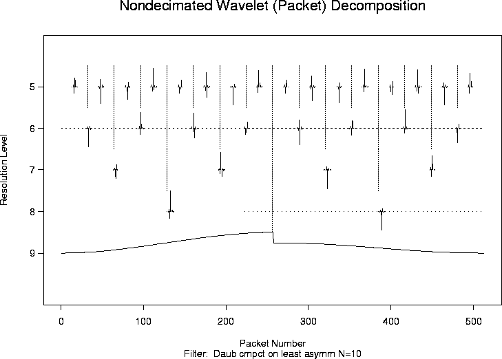 #
# The coefficients in this plot at each resolution level are the same
# as the ones in the non-decimated transform plot in the wd
# help page except they are in a different order. For more information
# about how the ordering works in each case see
# Nason, Sapatinas and Sawczenko, 1998.
#
# Next example
# ------------
# The chirp signal is also another good example to use.
#
#
# Generate some test data
#
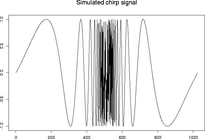
> test.chirp <- simchirp()$y
> tsplot(test.chirp, main="Simulated chirp signal")
#
# The coefficients in this plot at each resolution level are the same
# as the ones in the non-decimated transform plot in the wd
# help page except they are in a different order. For more information
# about how the ordering works in each case see
# Nason, Sapatinas and Sawczenko, 1998.
#
# Next example
# ------------
# The chirp signal is also another good example to use.
#
#
# Generate some test data
#
> test.chirp <- simchirp()$y
> tsplot(test.chirp, main="Simulated chirp signal")
 #
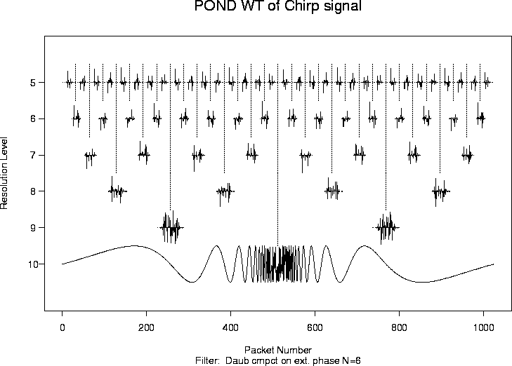
# Now let's do the packet-ordered non-decimated wavelet transform.
# For a change let's use Daubechies extremal phase wavelet with 6
# vanishing moments (a totally arbitrary choice, please don't read
# anything into it).
#
> chirpwst <- wst(test.chirp, filter.number=6, family="DaubExPhase")
> plot(chirpwst, main="POND WT of Chirp signal")
#
# Now let's do the packet-ordered non-decimated wavelet transform.
# For a change let's use Daubechies extremal phase wavelet with 6
# vanishing moments (a totally arbitrary choice, please don't read
# anything into it).
#
> chirpwst <- wst(test.chirp, filter.number=6, family="DaubExPhase")
> plot(chirpwst, main="POND WT of Chirp signal")

 #
# Now let's do the packet-ordered non-decimated wavelet transform.
#
> TDwst <- wst(test.data)
#
# And let's plot it....
#
> plot(TDwst)
#
# Now let's do the packet-ordered non-decimated wavelet transform.
#
> TDwst <- wst(test.data)
#
# And let's plot it....
#
> plot(TDwst)
 #
# The coefficients in this plot at each resolution level are the same
# as the ones in the non-decimated transform plot in the wd
# help page except they are in a different order. For more information
# about how the ordering works in each case see
# Nason, Sapatinas and Sawczenko, 1998.
#
# Next example
# ------------
# The chirp signal is also another good example to use.
#
#
# Generate some test data
#
> test.chirp <- simchirp()$y
> tsplot(test.chirp, main="Simulated chirp signal")
#
# The coefficients in this plot at each resolution level are the same
# as the ones in the non-decimated transform plot in the wd
# help page except they are in a different order. For more information
# about how the ordering works in each case see
# Nason, Sapatinas and Sawczenko, 1998.
#
# Next example
# ------------
# The chirp signal is also another good example to use.
#
#
# Generate some test data
#
> test.chirp <- simchirp()$y
> tsplot(test.chirp, main="Simulated chirp signal")
 #
# Now let's do the packet-ordered non-decimated wavelet transform.
# For a change let's use Daubechies extremal phase wavelet with 6
# vanishing moments (a totally arbitrary choice, please don't read
# anything into it).
#
> chirpwst <- wst(test.chirp, filter.number=6, family="DaubExPhase")
> plot(chirpwst, main="POND WT of Chirp signal")
#
# Now let's do the packet-ordered non-decimated wavelet transform.
# For a change let's use Daubechies extremal phase wavelet with 6
# vanishing moments (a totally arbitrary choice, please don't read
# anything into it).
#
> chirpwst <- wst(test.chirp, filter.number=6, family="DaubExPhase")
> plot(chirpwst, main="POND WT of Chirp signal")
