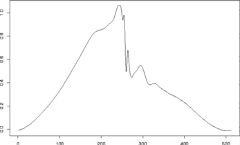
The default of levels = 3:(wd$nlevels - 1) for the
levels option most certainly does not work globally for
all data problems and situations. The level at which thresholding begins
(i.e. the given threshold and finer scale wavelets) is called the
primary resolution and is unique to a particular problem.
In some ways choice of the primary resolution is very similar to choosing
the bandwidth in kernel regression albeit on a logarithmic scale.
See Hall and Patil, (1995) and
Hall and Nason (1997) for more information.
For each data problem you need to work out which is the best
primary resolution. This can be done by gaining experience at what works
best, or using prior knowledge. It is possible to "automatically" choose
a "best" primary resolution using cross-validation (but not in WaveThresh).
Secondly the levels argument computes and applies the threshold at the
levels specified in the levels argument. It does this for
all the levels specified. Sometimes, in wavelet shrinkage, the threshold
is computed using only the finest scale coefficients (or more precisely
the estimate of the overall noise level). If you want your threshold
variance estimate only to use the finest scale coefficients (e.g.
with universal thresholding) then you will have to apply the
threshold.wd function twice. Once (with levels set equal to
nlevels(wd)-1 and with
return.threshold=TRUE to return the threshold computed on
the finest scale and then apply the threshold function with the
manual option supplying the value of the previously computed
threshold as the value options.
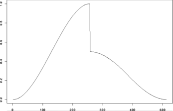 #
# Generate some noisy data
#
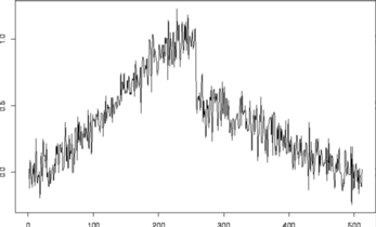
ynoise <- test.data + rnorm(512, sd=0.1)
#
# Plot it
#
tsplot(ynoise)
#
# Generate some noisy data
#
ynoise <- test.data + rnorm(512, sd=0.1)
#
# Plot it
#
tsplot(ynoise)
 #
# Now take the discrete wavelet transform
# N.b. I have no idea if the default wavelets here are appropriate for
# this particular example.
#
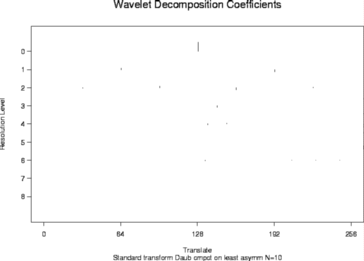
ynwd <- wd(ynoise)
plot(ynwd)
#
# Now take the discrete wavelet transform
# N.b. I have no idea if the default wavelets here are appropriate for
# this particular example.
#
ynwd <- wd(ynoise)
plot(ynwd)
 #
# Now do thresholding. We'll use a universal policy,
# and madmad deviance estimate on the finest
# coefficients and return the threshold. We'll also get it to be verbose
# so we can watch the process.
#
ynwdT1 <- threshold(ynwd, policy="universal", dev=madmad,
levels= nlevels(ynwd)-1, return.threshold=TRUE,
verbose=TRUE)
# threshold.wd:
# Argument checking
# Universal policy...All levels at once
# Global threshold is: 0.328410967430135
#
# Why is this the threshold? Well in this case n=512 so sqrt(2*log(n)),
# the universal threshold,
# is equal to 3.53223. Since the noise is about 0.1 (because that's what
# we generated it to be) the threshold is about 0.353.
#
# Now let's apply this threshold to all levels in the noisy wavelet object
#
ynwdT1obj <- threshold(ynwd, policy="manual", value=ynwdT1,
levels=0:(nlevels(ynwd)-1))
#
# And let's plot it
#
plot(ynwdT1obj)
#
# Now do thresholding. We'll use a universal policy,
# and madmad deviance estimate on the finest
# coefficients and return the threshold. We'll also get it to be verbose
# so we can watch the process.
#
ynwdT1 <- threshold(ynwd, policy="universal", dev=madmad,
levels= nlevels(ynwd)-1, return.threshold=TRUE,
verbose=TRUE)
# threshold.wd:
# Argument checking
# Universal policy...All levels at once
# Global threshold is: 0.328410967430135
#
# Why is this the threshold? Well in this case n=512 so sqrt(2*log(n)),
# the universal threshold,
# is equal to 3.53223. Since the noise is about 0.1 (because that's what
# we generated it to be) the threshold is about 0.353.
#
# Now let's apply this threshold to all levels in the noisy wavelet object
#
ynwdT1obj <- threshold(ynwd, policy="manual", value=ynwdT1,
levels=0:(nlevels(ynwd)-1))
#
# And let's plot it
#
plot(ynwdT1obj)
 #
# You'll see that a lot of coefficients have been set to zero, or shrunk.
#
# Let's try a Bayesian example this time!
#
ynwdT2obj <- threshold(ynwd, policy="BayesThresh")
#
# And plot the coefficients
#
plot(ynwdT2obj)
#
# You'll see that a lot of coefficients have been set to zero, or shrunk.
#
# Let's try a Bayesian example this time!
#
ynwdT2obj <- threshold(ynwd, policy="BayesThresh")
#
# And plot the coefficients
#
plot(ynwdT2obj)
 #
# Let us now see what the actual estimates look like
#
ywr1 <- wr(ynwdT1obj)
ywr2 <- wr(ynwdT2obj)
#
# Here's the estimate using universal thresholding
#
tsplot(ywr1)
#
# Let us now see what the actual estimates look like
#
ywr1 <- wr(ynwdT1obj)
ywr2 <- wr(ynwdT2obj)
#
# Here's the estimate using universal thresholding
#
tsplot(ywr1)
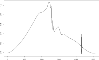 #
# Here's the estimate using BayesThresh
#
tsplot(ywr2)
#
# Here's the estimate using BayesThresh
#
tsplot(ywr2)
