WaveThresh
Help
plot.mwd
Use plot on an mwd object.
DESCRIPTION
Plots the wavelet coefficients of a mwd
class object.
USAGE
plot.mwd(mwd, first.level = 1, main = "Wavelet Decomposition Coefficients",
        scaling = "compensated", rhlab = F, sub = mwd$filter$name,
	NotPlotVal = 0.05, xlab = "Translate", ylab = "Resolutioin level",
	return.scale = T, colour = (2:(npsi + 1)), ...)
REQUIRED ARGUMENTS
- mwd
- The mwd object whose coefficients you wish to
plot.
OPTIONAL ARGUMENTS
-
first.level
- The first resolution level to begin plotting at. This argument can
be quite useful when you want to supress some of the coarser levels
in the diagram.
-
main
- The main title of the plot.
-
scaling
- How you want the coefficients to be scaled. The options are:
"global" - one scale factor is chosen for the whole plot.
The scale factor depends on the coefficient to be included on the
plot that has the largest absolute value. The global
option is useful when comparing coefficients that might appear anywhere
in the plot; "by.level" - a scale factor is chosen for
each resolution level in the plot. The scale factor for a level
depends on the coefficient in that level that has the largest
absolute value. The "by.level" option is useful when
you wish to compare coefficients within a resolution level.
The other option is "compensated"
which is the same as "global" except
for that finer scales' coefficients are scaled up by a factor
of SQRT(2) for compensated.
This latter options is sometimes useful.
-
rhlab
- If
T then a set of labels is produced on the right hand
axis. The axis labels in this case refer to the scale factors used
to scale each level and correspond to value of the largest coefficient
(in absolute value) in each scale
(when scaling=="by.level")
or absolutely (when scaling="global").
If the rhlab argument is F then no right
hand axis labels are produced.
-
sub
- A subtitle for the plot.
-
NotPlotVal
- Doesn't seem to be implemented.
-
xlab
- A title for the x-axis
-
ylab
- A title for the y-axis
-
return.scale
- If true (default) the scale for each resolution level is returned
-
colour
- A vector of length
mwd$npsi,
the values of which are the colours used
to plot the coefficients, one for each distinct type of wavelet (with
apologies to our American cousins for not spelling colour correctly!)
-
...
- other arguments to be supplied to plot.
VALUE
Axis labels for each resolution level unless return.scale=F
when NULL is returned. The axis values are the maximum
of the absolute value of the coefficients at that resolution level.
They are returned because they are sometimes hard to read on the plot.
SIDE EFFECTS
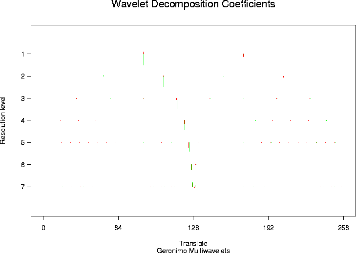
A plot of the coefficients contained within the mwd
object at each resolution level is produced.
DETAILS
Produces a plot similar to the ones in
Donoho and Johnstone, 1994.
Wavelet coefficients for each resolution level are
plotted
one above the other, with the high resolution coefficients at the
bottom, and the low resolution at the top.
Each vector is represented by mwd$npsi
lines one for each element in
the coefficient vector. If colour is supported by the device
each element will be represented by a different coulour.
The coefficients are
plotted using the segment
function, with a large positive coefficient
being plotted above an imaginary horizontal centre line, and a large
negative coefficient plotted below it. The position of a coefficient
along a line is indicative of the wavelet basis function's translate
number.
The resolution levels are labelled on the left-hand side axis,
and the maximum values of the absolute values of the coefficients
for the particular level form the right-hand side axis.
The levels of coefficients can be scaled in three ways. If you are
not interested in comparing the relative scales of coefficients
from different levels, then the default scaling option,
"by.level"
is what you need. This computes the maximum of the absolute value
of the coefficients at a particular level and scales the so that
the fit nicely onto the plot. For this option, each level is scaled
DIFFERENTLY.
To obtain a uniform scale for all the levels specify
the "global" option to the scaling argument.
This will allow you to make inter-level comparisons.
RELEASE
Version 3.9.6 (Although Copyright Tim Downie 1995-6).
SEE ALSO
accessC.mwd,
accessD.mwd,
draw.mwd,
mfirst.last,
mfilter.select,
mwd,
mwd object,
mwr,
print.mwd,
putC.mwd,
putD.mwd,
summary.mwd,
threshold.mwd,
wd,
wr.mwd.
EXAMPLES
#
# Generate some test data
#
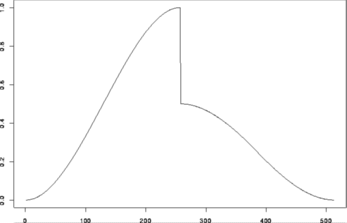
> test.data <- example.1()$y
> tsplot(test.data)
 #
# Decompose test.data with multiple wavelet transform and
# plot the wavelet coefficients
#
> tdmwd <- mwd(test.data)
> plot(tdmwd)
#
# Decompose test.data with multiple wavelet transform and
# plot the wavelet coefficients
#
> tdmwd <- mwd(test.data)
> plot(tdmwd)
 #[1] 1.851894 1.851894 1.851894 1.851894 1.851894 1.851894 1.851894
#
# You should see a plot with wavelet coefficients like in
# plot.wd but at each coefficient position
# there are two coefficients in two different colours one for each of
# the wavelets at that position.
#
# Note the scale for each level is returned by the function.
 #
# Decompose test.data with multiple wavelet transform and
# plot the wavelet coefficients
#
> tdmwd <- mwd(test.data)
> plot(tdmwd)
#
# Decompose test.data with multiple wavelet transform and
# plot the wavelet coefficients
#
> tdmwd <- mwd(test.data)
> plot(tdmwd)
 #[1] 1.851894 1.851894 1.851894 1.851894 1.851894 1.851894 1.851894
#
# You should see a plot with wavelet coefficients like in
# plot.wd but at each coefficient position
# there are two coefficients in two different colours one for each of
# the wavelets at that position.
#
# Note the scale for each level is returned by the function.