WaveThresh
Help
threshold.mwd
Use threshold on an mwd object.
DESCRIPTION
Applies hard or soft thresholding to multiple wavelet decomposition object
mwd.object.
USAGE
threshold.mwd(mwd, levels = 3:(mwd$nlevels - 1), type = "hard",
	policy = "universal", boundary = F, verbose = F, return.threshold = F,
	threshold = 0, covtol = 1e-09, robust = T, return.chisq = F,
	bivariate = T)
REQUIRED ARGUMENTS
- mwd
- The multiple wavelet decomposition object that you wish to threshold.
OPTIONAL ARGUMENTS
-
levels
- a vector of integers which determines which scale levels are thresholded
in the decomposition. Each integer in the vector must refer to a valid
level in the mwd object supplied. This is usually
any integer from 0 to
nlevels(wd)-1 inclusive.
Only the levels in this vector contribute to the computation of the
threshold and its application.
-
type
- determines the type of thresholding this can be
"hard"
or "soft".
-
policy
- selects the technique by which the threshold value is selected. Each
policy corresponds to a method in the literature. At present the
different policies are
"universal",
"manual",
"single".
The policies are described in detail below.
-
boundary
- If this argument is
TRUE
then the boundary bookeeping values are
included for thresholding, otherwise they are not.
-
verbose
- if
TRUE
then the function prints out informative messages as it progresses.
-
return.threshold
- If this option is
TRUE then the actual
value of the threshold
is returned. If this option is FALSE then a thresholded version of the
input is returned.
-
threshold
- This argument conveys the user supplied threshold. If the
policy="manual"
then value is the actual
threshold value. Any other policy means that the
threshold value is ignored.
-
covtol
- The tolerance for what constitutes a singular variance matrix.
If smallest eigenvalue of the estimated variance matrix is
less than
covtol
then it is assumed to be singular and no thresholing is done
at that level.
Note: do not confuse covtol with cvtol
an argument in threshold.wd.
-
robust
- If true the variance matrix at each level is estimated using a robust
method (mad) otherwise it is estimated using var().
-
return.chisq
- If true the vector of values to be thresholded is returned.
These values are a quadratic form of each coefficient vector,
and under normal assumptions the noise
component will have a chi-squared distribution
(see Downie and Silverman 1996).
VALUE
An object of class mwd. This object contains the
thresholded wavelet coefficients. Note that if the
return.threshold option is set to TRUE then the threshold
values will be returned, or if
return.chisq the vector of values to be thresholded will be
returned,
rather than the thresholded object.
SIDE EFFECTS
None
DETAILS
Thresholding modifies the coefficients within a
mwd object. The modification can be performed either
with a "hard" or "soft" thresholding selected by the
type argument.
Unless policy="single", the following method is applied.
The columns of mwd$D are taken as coefficient vectors D_j,k.
From these chisq_j,k=D_j,k . V_j^-1 . D_j,k is computed, where V_j^-1
is the inverse of the estimated variance of the coefficient vectors in
that level (j). Chisq_j,k is a positive scalar which is to be thresholded
in a similar manner to univariate hard or soft thresholding.
To obtain the new values of D_j,k shrink the vector by the same proportion
as was the corresponding chisq_j,k term.
- single
- If
policy="single"
then univariate thresholding is applied to each element of D as in
(Strela et al 1999).
- universal
- The
universal threshold is computed using 2log(n)
(See Downie & Silverman 1996)
where n is the number of coefficient vectors to be thresholded.
- manual
- The
"manual" policy is simple.
You supply a threshold value to the threshold argument
and hard or soft
thresholding is performed using that value.
RELEASE
Version 3.9.6 (Although Copyright Tim Downie 1995-6).
SEE ALSO
accessC.mwd,
accessD.mwd,
draw.mwd,
mfirst.last,
mfilter.select,
mwd,
mwd object,
mwr,
plot.mwd,
print.mwd,
putC.mwd,
putD.mwd,
summary.mwd,
wd,
wr.mwd.
#
# Generate some test data
#
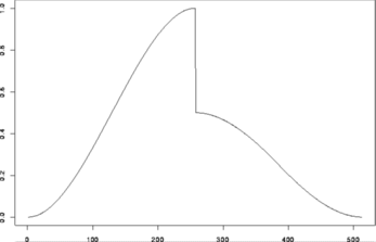
test.data <- example.1()$y
tsplot(test.data)
 #
# Generate some noisy data
#
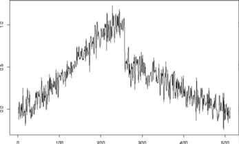
ynoise <- test.data + rnorm(512, sd=0.1)
#
# Plot it
#
tsplot(ynoise)
#
# Generate some noisy data
#
ynoise <- test.data + rnorm(512, sd=0.1)
#
# Plot it
#
tsplot(ynoise)
 #
# Now take the discrete multiple wavelet transform
# N.b. I have no idea if the default wavelets here are appropriate for
# this particular example.
#
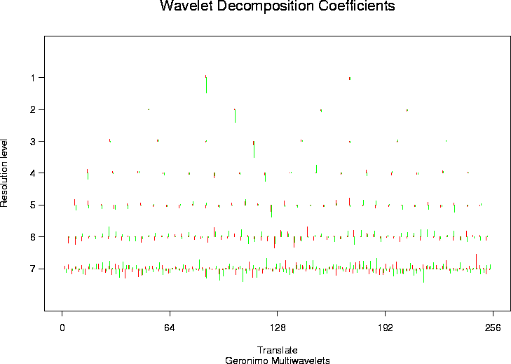
ynmwd <- mwd(ynoise)
plot(ynwd)
#
# Now take the discrete multiple wavelet transform
# N.b. I have no idea if the default wavelets here are appropriate for
# this particular example.
#
ynmwd <- mwd(ynoise)
plot(ynwd)
 # [1] 2.020681 2.020681 2.020681 2.020681 2.020681 2.020681 2.020681
#
# Now do thresholding. We'll use the default arguments.
#
ynmwdT <- threshold(ynmwd)
#
# And let's plot it
#
plot(ynmwdT)
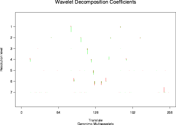 #
# Let us now see what the actual estimate looks like
#
ymwr <- wr(ynwdT)
#
# Here's the estimate...
#
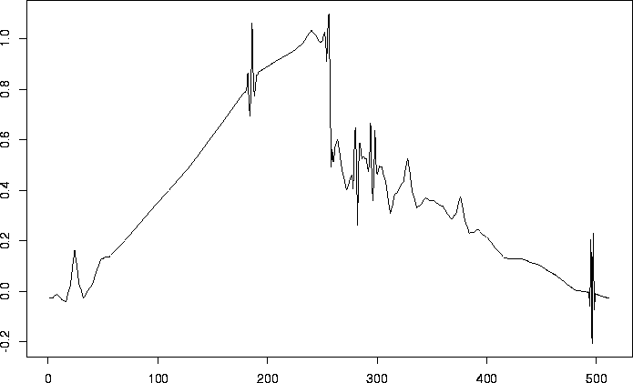
tsplot(ywr1)
#
# Let us now see what the actual estimate looks like
#
ymwr <- wr(ynwdT)
#
# Here's the estimate...
#
tsplot(ywr1)

 #
# Generate some noisy data
#
ynoise <- test.data + rnorm(512, sd=0.1)
#
# Plot it
#
tsplot(ynoise)
#
# Generate some noisy data
#
ynoise <- test.data + rnorm(512, sd=0.1)
#
# Plot it
#
tsplot(ynoise)
 #
# Now take the discrete multiple wavelet transform
# N.b. I have no idea if the default wavelets here are appropriate for
# this particular example.
#
ynmwd <- mwd(ynoise)
plot(ynwd)
#
# Now take the discrete multiple wavelet transform
# N.b. I have no idea if the default wavelets here are appropriate for
# this particular example.
#
ynmwd <- mwd(ynoise)
plot(ynwd)
 # [1] 2.020681 2.020681 2.020681 2.020681 2.020681 2.020681 2.020681
#
# Now do thresholding. We'll use the default arguments.
#
ynmwdT <- threshold(ynmwd)
#
# And let's plot it
#
plot(ynmwdT)
 #
# Let us now see what the actual estimate looks like
#
ymwr <- wr(ynwdT)
#
# Here's the estimate...
#
tsplot(ywr1)
#
# Let us now see what the actual estimate looks like
#
ymwr <- wr(ynwdT)
#
# Here's the estimate...
#
tsplot(ywr1)
